Lecture 1: Introduction and ‘Atomos’
0) Orientation: How this course works and what to expect
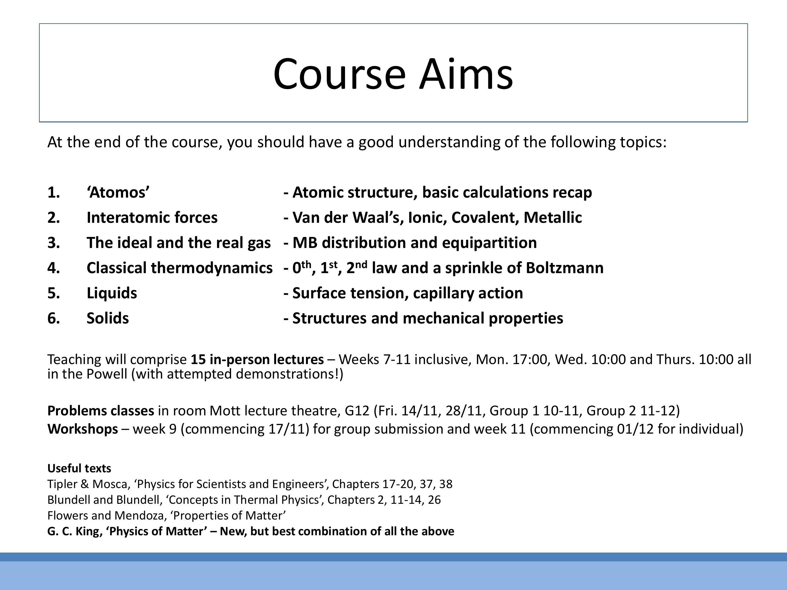
This course, Properties of Matter (PoM), is taught by Dr Ross Springell, an Associate Professor in the School of Physics. While you may be familiar with mechanics, this course shifts focus to understanding systems containing many particles, such as gases, liquids, and solids. Dr Springell's research background is in solid-state and condensed matter physics, particularly with heavy elements like actinides, and includes applications in nuclear fuels, waste, and tritium storage.
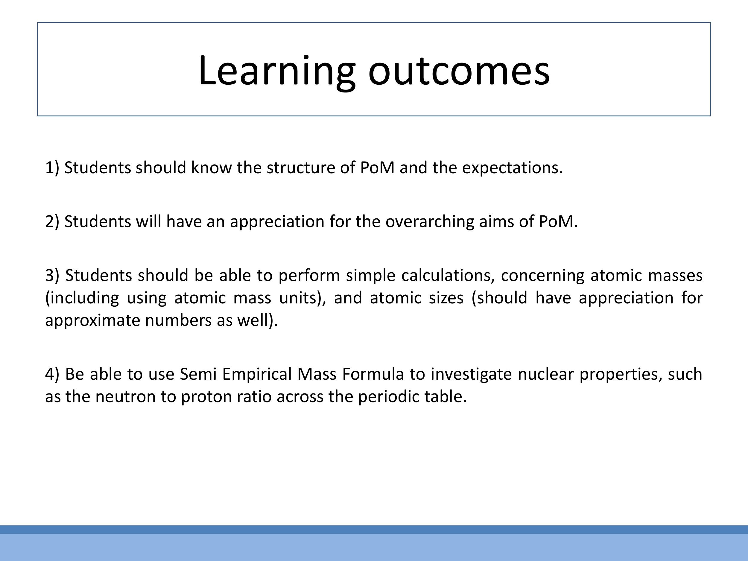
Unlike some other courses, pre-written lecture notes will not be provided. You are expected to maintain your own notes during lectures. However, the lecture slides and handwritten derivations shown in class will be uploaded to Blackboard after each session. Each lecture begins with a slide outlining the learning outcomes, which serve as a guide but won't be read out in detail during the lecture itself. The course content has been slightly reduced this year based on previous feedback.
For further reading, several textbooks are recommended: Tipler & Mosca, Blundell & Blundell, and Flowers & Mendoza. G. C. King's "Physics of Matter" is particularly recommended as it aligns closely with the course content, though an eBook version is not currently available. This introductory lecture contains mostly non-examinable material. However, you are expected to be able to perform basic calculations involving atomic masses, moles, and atomic sizes.
⚠️ Exam Alert! The lecturer explicitly stated: "Sometimes I'll give away easter eggs, perhaps as to what might be in the exam... in order to give some advantage, at least to those that turn up to the lectures." This means attending lectures can provide insights into examinable content.
Materials and condensed matter physics is a vast and active research area, offering numerous career opportunities. Students interested in this field can explore summer internships (often for those in their penultimate year), MSc programmes in Nuclear Science & Engineering, or PhD positions. Information on these opportunities is often posted on the third-floor noticeboard.
1) From single-particle mechanics to many-body physics
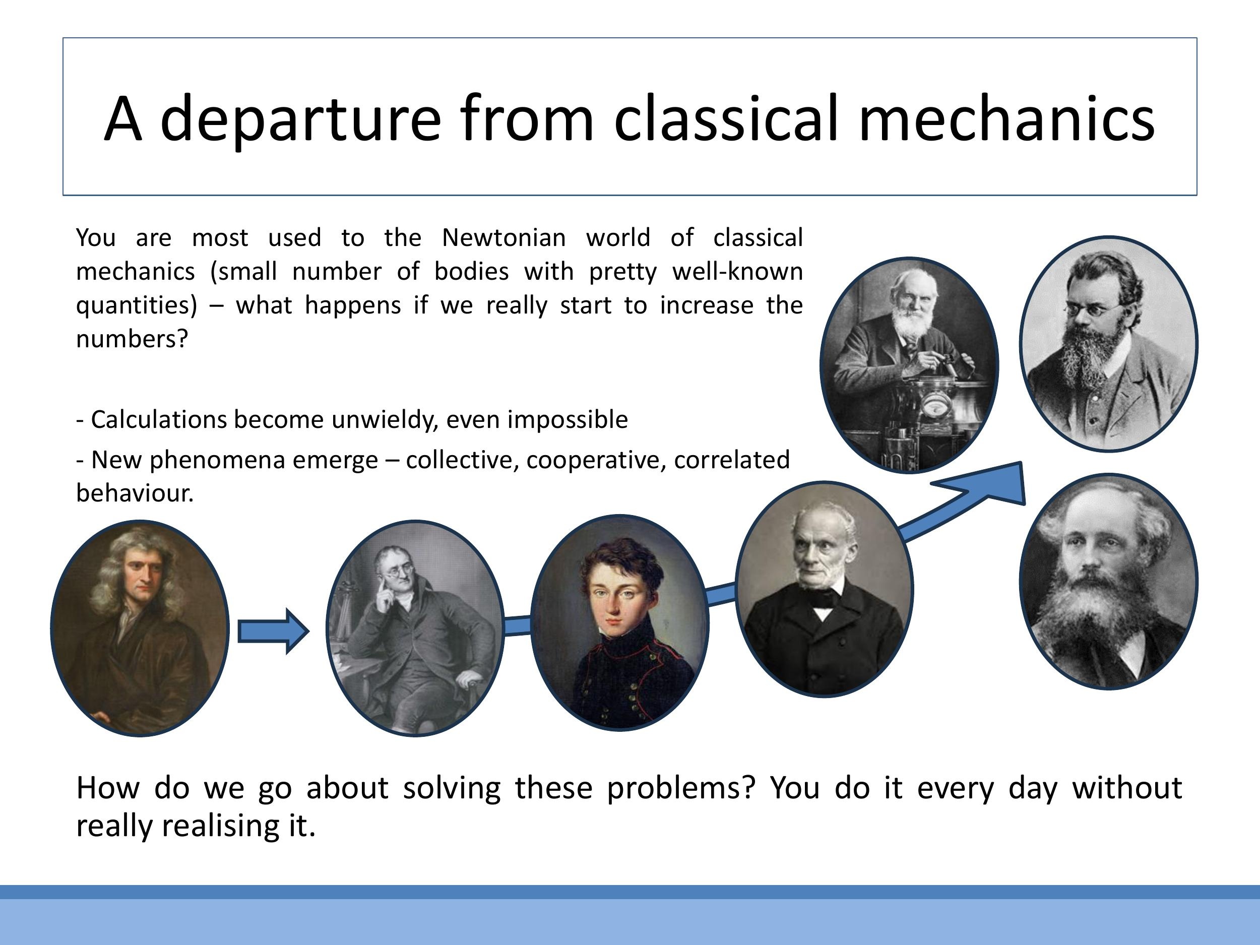
This course represents a significant shift from the classical mechanics you may be used to, which typically deals with a small number of particles or bodies with well-defined initial conditions, such as projectile motion. When dealing with real materials and macroscopic matter, like the air in a room or atoms in a solid, the number of particles is astronomically large. Tracking the individual behaviour of each particle becomes an impossible task due to the sheer number of degrees of freedom involved.
To address this "many-body problem," we adopt new strategies. Instead of focusing on individual particles, we use averaged, emergent quantities to describe the system's collective behaviour. Temperature is a perfect example: we use it daily to describe the average kinetic energy of countless particles without explicitly tracking each one. This approach allows us to understand emergent phenomena, which are complex, large-scale behaviours that arise from the interactions of many individual components and are not predictable from the properties of single constituents alone.
Historically, the scientific trajectory reflects this shift. Early deterministic approaches by figures like Newton and Laplace focused on few-body systems. However, the Industrial Revolution's need to optimise steam engines drove the development of thermodynamics. This led to pioneers like Fourier (heat transfer), Clausius (entropy), Maxwell (molecular speed distributions), Boltzmann (statistical mechanics), and Kelvin (absolute temperature) establishing the tools needed to describe many-body systems.
2) Emergence in practice: intuition before equations
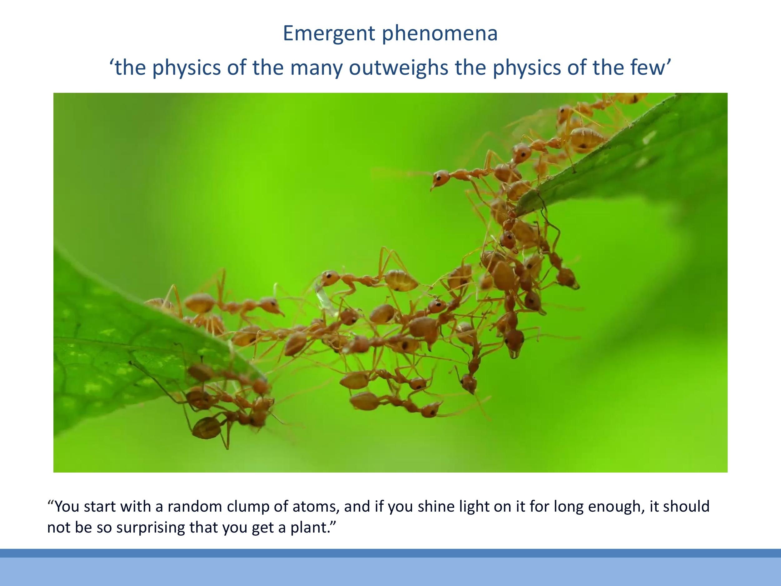
Collective behaviour illustrates how many interacting units can produce stable, large-scale patterns that are not predictable by modelling one unit alone. For example, a murmuration of starlings forms intricate, coordinated aerial displays that no computational model of individual birds could foresee. Similarly, ants can cooperate to build living bridges, as shown in the image, where individual ants link together to span gaps. This biological example helps build an intuition for emergence without immediately diving into complex mathematics.
This same principle applies directly to physical materials. The electronic, magnetic, and superconducting properties that we observe in matter arise from the collective behaviour of countless electrons and the atomic-scale interactions between them. Understanding these emergent properties, where the whole is greater than the sum of its parts, is fundamental to the study of the Properties of Matter. This course will focus on building this physical understanding before formalising it with equations.
3) Demonstrations of thermodynamic and collective transitions
3.1 Ferromagnetism and the Curie temperature (Nickel + magnet + heat)
We can observe emergent phenomena through simple demonstrations. Consider a piece of nickel, an elemental ferromagnet, attracted to a permanent magnet at room temperature. When the nickel is heated with a flame, it detaches from the magnet. As it cools in the air, it reattaches, creating an oscillation. This happens because ferromagnets are composed of many microscopic magnetic moments that align collectively, leading to a strong attraction. Heating injects thermal energy into the material, which randomises these moments above a specific point called the Curie temperature. Above this temperature, the material transitions from a ferromagnetic (ordered, strongly attractive) state to a paramagnetic (disordered, weakly attractive) state. This is a reversible thermodynamic transition driven by temperature.
Another striking example is a shape-memory alloy. If you deform a paperclip made from such an alloy into a random shape, it will instantly return to its original "remembered" form when placed in hot water. This phenomenon is due to a thermodynamic phase transition between two crystal structures. At low temperatures, the alloy exists in a phase that can easily accommodate deformation without breaking atomic bonds; instead, it rearranges internal "twin" structures. When heated, it transitions to a high-temperature cubic phase with a single preferred configuration, forcing it back to the shape it was originally formed in.
3.3 Type II superconductivity and flux pinning (YBCO + magnet + liquid nitrogen)
A dramatic demonstration of collective behaviour is quantum levitation using a Type II superconductor. When a YBCO (Yttrium Barium Copper Oxide) ceramic puck is cooled below its transition temperature (around $92 \, \text{K} $) with liquid nitrogen ($ 77 \, \text{K} $), a small magnet placed above it will levitate and become "pinned" in position. This means the magnet is locked and can even be inverted without falling. Superconductors exhibit zero electrical resistance and strong diamagnetism (the Meissner effect), expelling magnetic fields. However, Type II superconductors allow quantised magnetic flux lines to penetrate through discrete, non-superconducting regions. These flux lines become trapped or "pinned" within the material, stabilising the levitation and fixing the magnet's relative position. The discovery of these "high-temperature" superconductors (superconducting above $ 77 \, \text{K}$) was significant because liquid nitrogen is much cheaper than liquid helium. The precise mechanism behind this type of superconductivity is still an active area of research.
4) The atomic picture: a brief historical scaffold
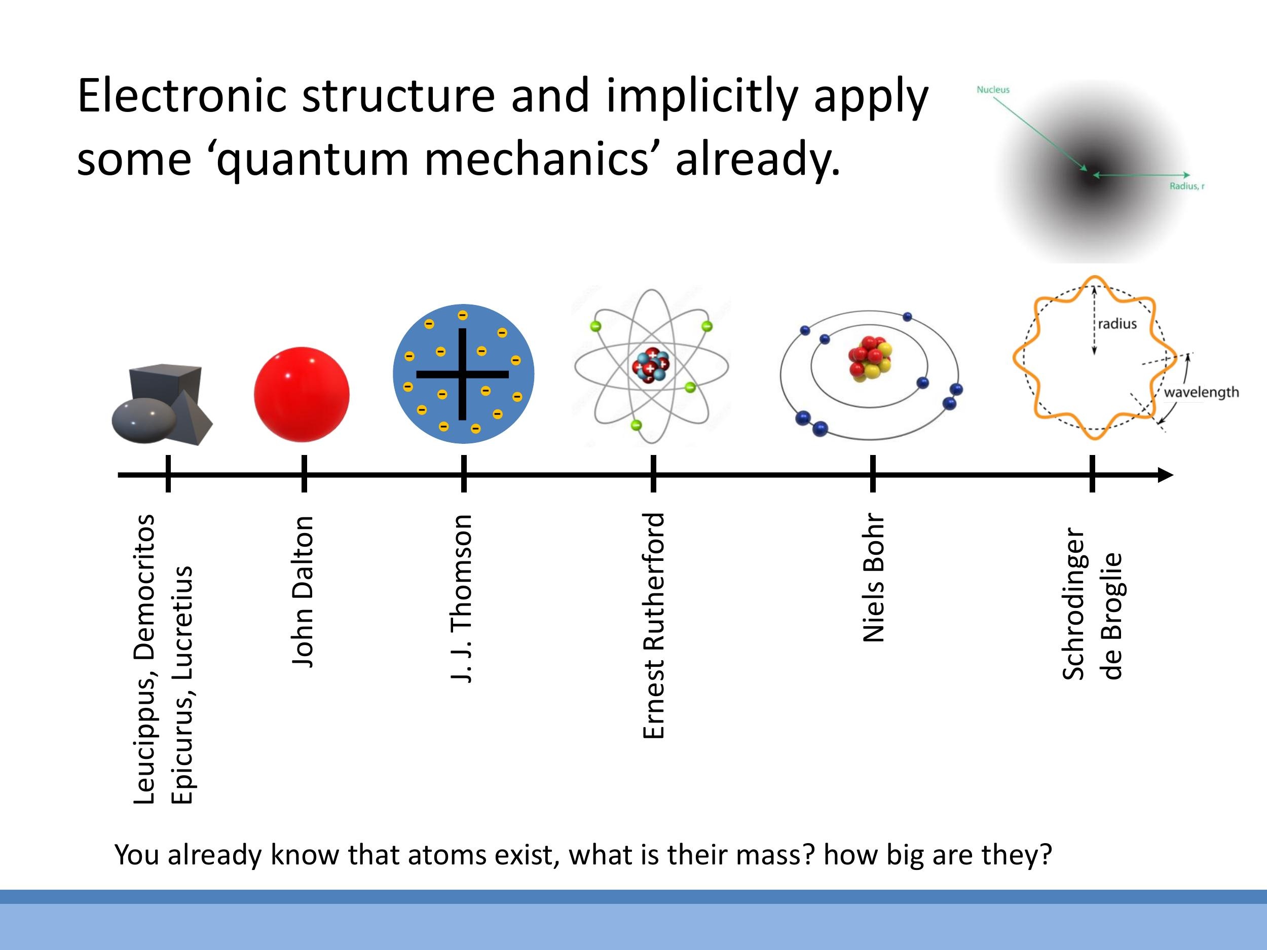
Our understanding of the atom has evolved significantly over time. Beginning with the philosophical concept of "atomos" (indivisible particles) from ancient Greek thinkers like Leucippus and Democritus, the modern atomic picture began to take shape with John Dalton's atomic theory in the early $19^\text{th}$ century. This was followed by J. J. Thomson's "plum pudding" model, which posited a positively charged sphere with embedded electrons. Ernest Rutherford's gold foil experiment then revealed the existence of a small, dense, positively charged nucleus, leading to the nuclear atom model. Niels Bohr further refined this with his model of electrons orbiting the nucleus in quantised energy levels.
The modern view of the atom, however, is rooted in quantum mechanics, building on the work of Schrödinger and de Broglie. In this picture, electrons are not tiny particles orbiting a nucleus, but rather wave-like entities that exist in probabilistic orbitals or "clouds" around the nucleus. These orbitals correspond to discrete energy levels. The nucleus itself is composed of protons and neutrons, and its properties are described by nuclear physics. While Bohr's model provides a useful conceptual stepping stone, the wave-mechanical and probabilistic description offers a more accurate representation of electron behaviour.
5) Quantitative foundations: mass, moles, and atomic size
5.1 Atomic mass units and isotopes
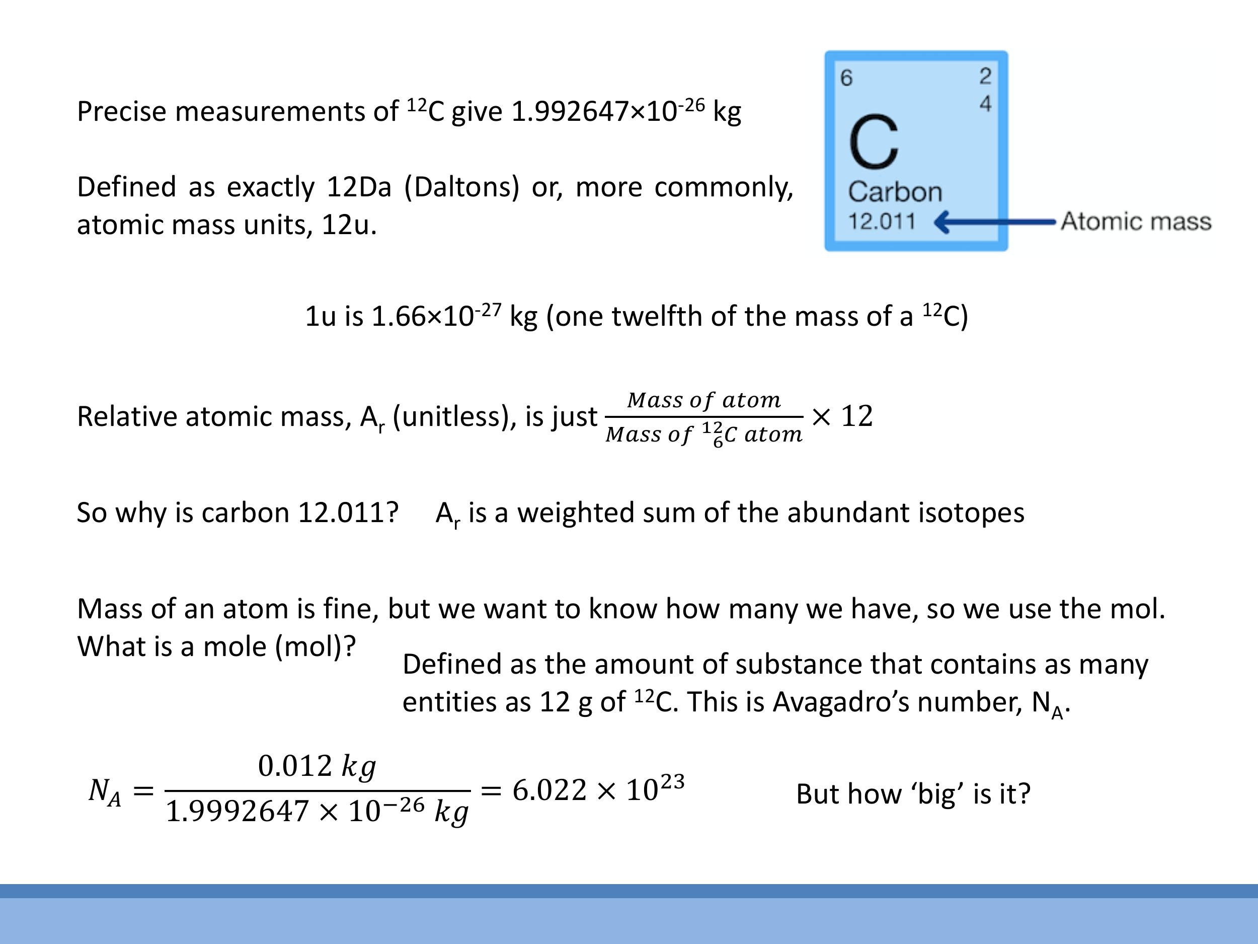
To quantify matter at the atomic scale, we use the atomic mass unit ($\text{u}$), also known as the Dalton ($\text{Da}$). This unit is precisely defined based on the carbon-12 ($^{12}\text{C}$) atom: one $^{12}\text{C}$ atom has a mass of exactly $12 \, \text{u} $. From this, we know that $ 1 \, \text{u} \approx 1.66 \times 10^{-27} \, \text{kg} $. The relative atomic mass ($ A_r $) is a unitless quantity that compares the mass of an atom to $ 1/12^\text{th} $ the mass of a $ ^{12}\text{C}$ atom:
$$
A_r = \frac{\text{Mass of atom}}{\text{Mass of } ^{12}\text{C atom}} \times 12
$$
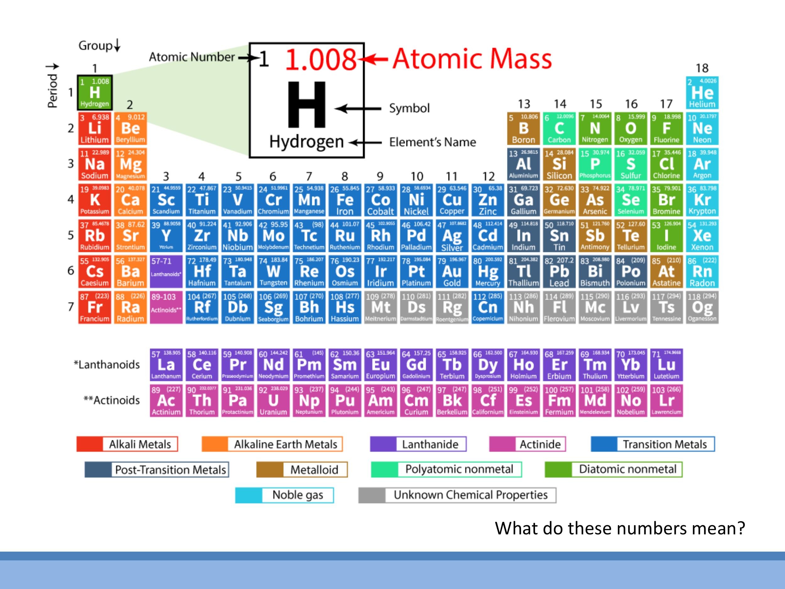
The atomic masses listed on the periodic table, such as carbon's $12.011$, are often non-integers. This is because most elements exist naturally as a mixture of different isotopes, which are atoms with the same number of protons but different numbers of neutrons. The listed atomic mass is a weighted average of the masses of these isotopes, taking into account their natural abundance. For example, carbon's $12.011$ reflects the natural abundance of $^{12}\text{C}$ and $^{13}\text{C}$.
5.2 Counting particles: the mole and Avogadro’s number
When dealing with macroscopic quantities of matter, we use the mole ($\text{mol}$) to count particles. One mole is defined as the amount of substance that contains as many elementary entities (atoms, molecules, etc.) as there are atoms in exactly $12 \, \text{g} $ of $ ^{12}\text{C} $. This definition directly leads to Avogadro's number ($ N_A$), which is the number of entities in one mole:
$$
N_A = \frac{0.012\,\text{kg}}{\text{mass of one } ^{12}\text{C atom}} \approx 6.022 \times 10^{23}\,\text{mol}^{-1}
$$
Avogadro's number is crucial because it provides a link between macroscopic quantities that we can measure (like grams or cubic centimetres) and the microscopic count of atoms or molecules.
5.3 Estimating how big an atom is (simple cubic packing model)
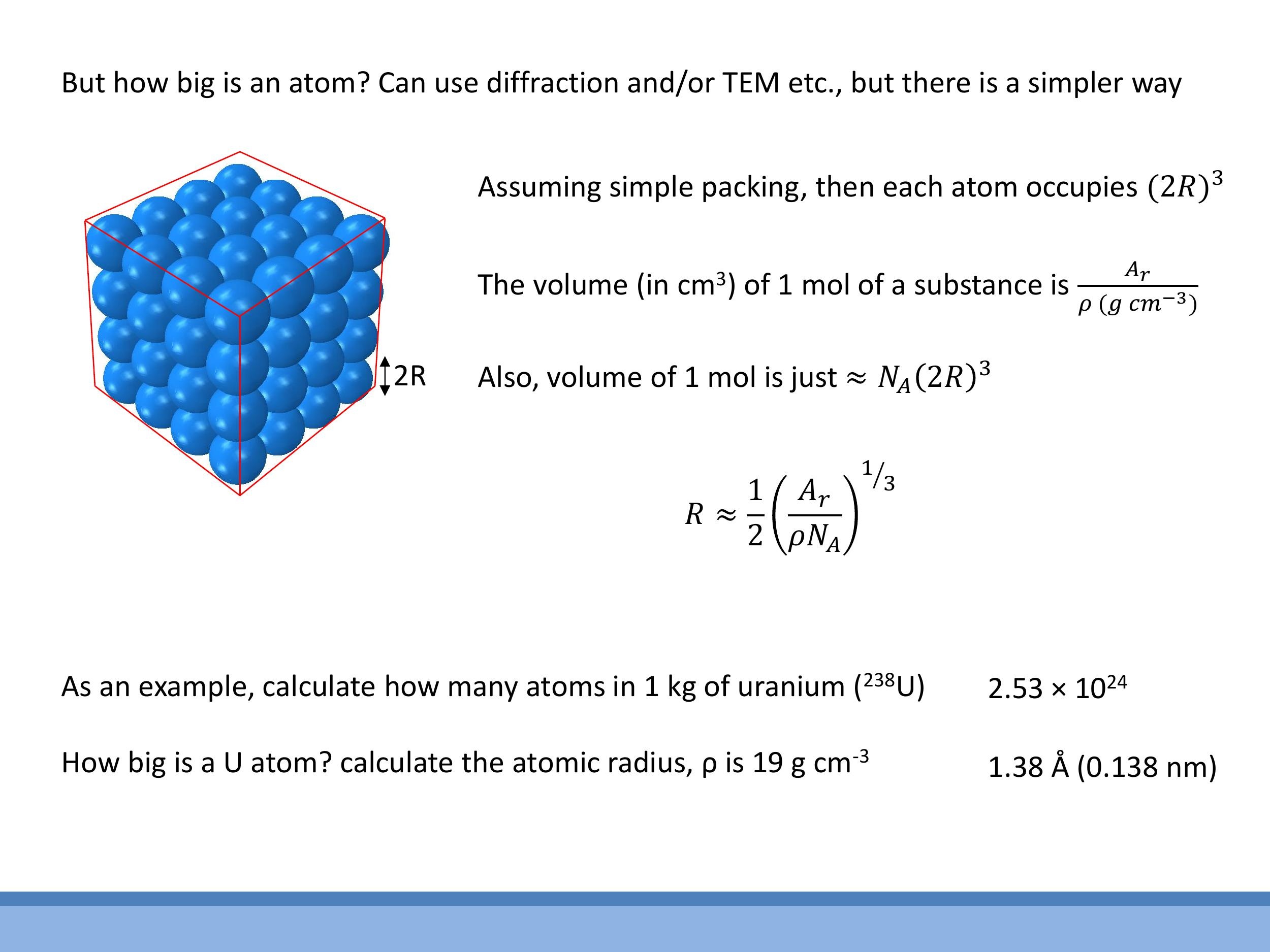
We can estimate the size of an atom using a simple "back-of-the-envelope" calculation, which is often surprisingly effective. In this model, we treat atoms as hard spheres of radius $R$ and assume they are packed in a simple cubic lattice. In this arrangement, each atom effectively occupies a cubic volume with side length $2R$, so the volume per atom is $(2R)^3$.
To connect this microscopic picture to macroscopic data, we can calculate the molar volume ($V_m$) from a substance's relative atomic mass ($A_r$, in $\text{g} \, \text{mol}^{-1} $) and its bulk density ($ \rho $, in $ \text{g} \, \text{cm}^{-3} $): $ V_m = A_r / \rho $. We also know that the molar volume is approximately the volume per atom multiplied by Avogadro's number: $ V_m \approx N_A (2R)^3 $. Equating these two expressions for molar volume allows us to solve for the atomic radius $ R$:
$$
R \approx \frac{1}{2} \left( \frac{A_r}{\rho N_A} \right)^{1/3}
$$
As an example, let's estimate the radius of a uranium atom. Given its relative atomic mass $A_r = 238 \, \text{g} \, \text{mol}^{-1} $ and density $ \rho = 19 \, \text{g} \, \text{cm}^{-3} $, the formula yields an atomic radius of $ R \approx 1.38 \, \text{Å} $ (or $ 0.138 \, \text{nm} $). This crude model provides a result remarkably close to experimental values, which are typically around $ 1.75 \, \text{Å}$, demonstrating the power and utility of such approximate models in physics. Being comfortable with these kinds of estimations and back-of-the-envelope reasoning is a valuable skill in this course.
6) The modelling mindset: “close enough” is often powerful
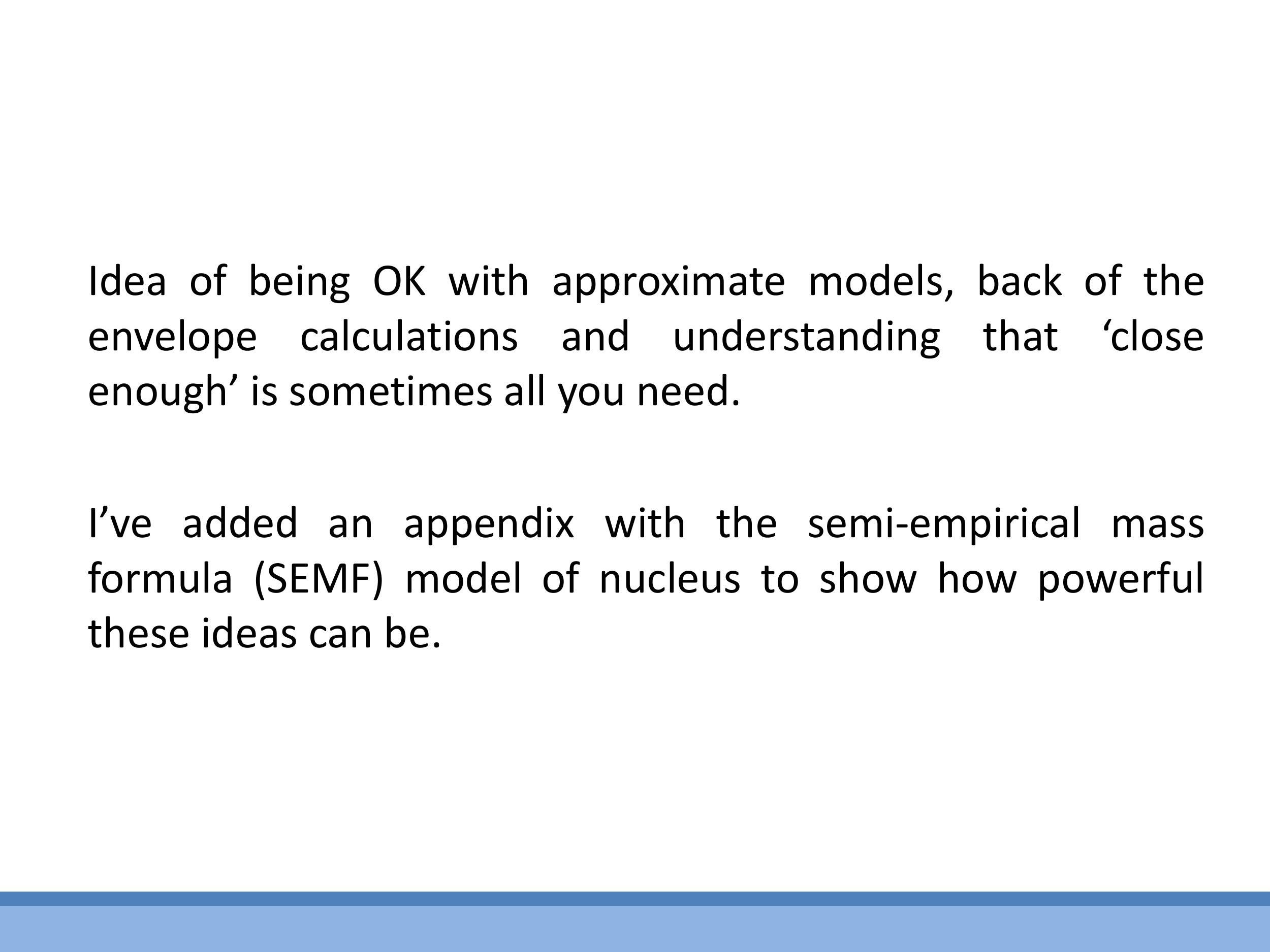
In physics, it's not always necessary to have exact microscopic detail to solve a problem. Often, a well-chosen, simplified model, coupled with reasonable approximations, can produce incredibly useful and testable estimates. This "close enough" approach allows us to gain quick physical insight and is a core problem-solving strategy in Properties of Matter. Throughout this course, we will frequently link macroscopic observables to microscopic models with simplifying assumptions, then sanity-check our results against experimental data. This iterative process of estimation, comparison, and refinement is fundamental to scientific discovery.
Appendix: Semi-empirical Mass Formula (SEMF)
Side Note: This material is supplementary and won't be examined, but provides useful context.
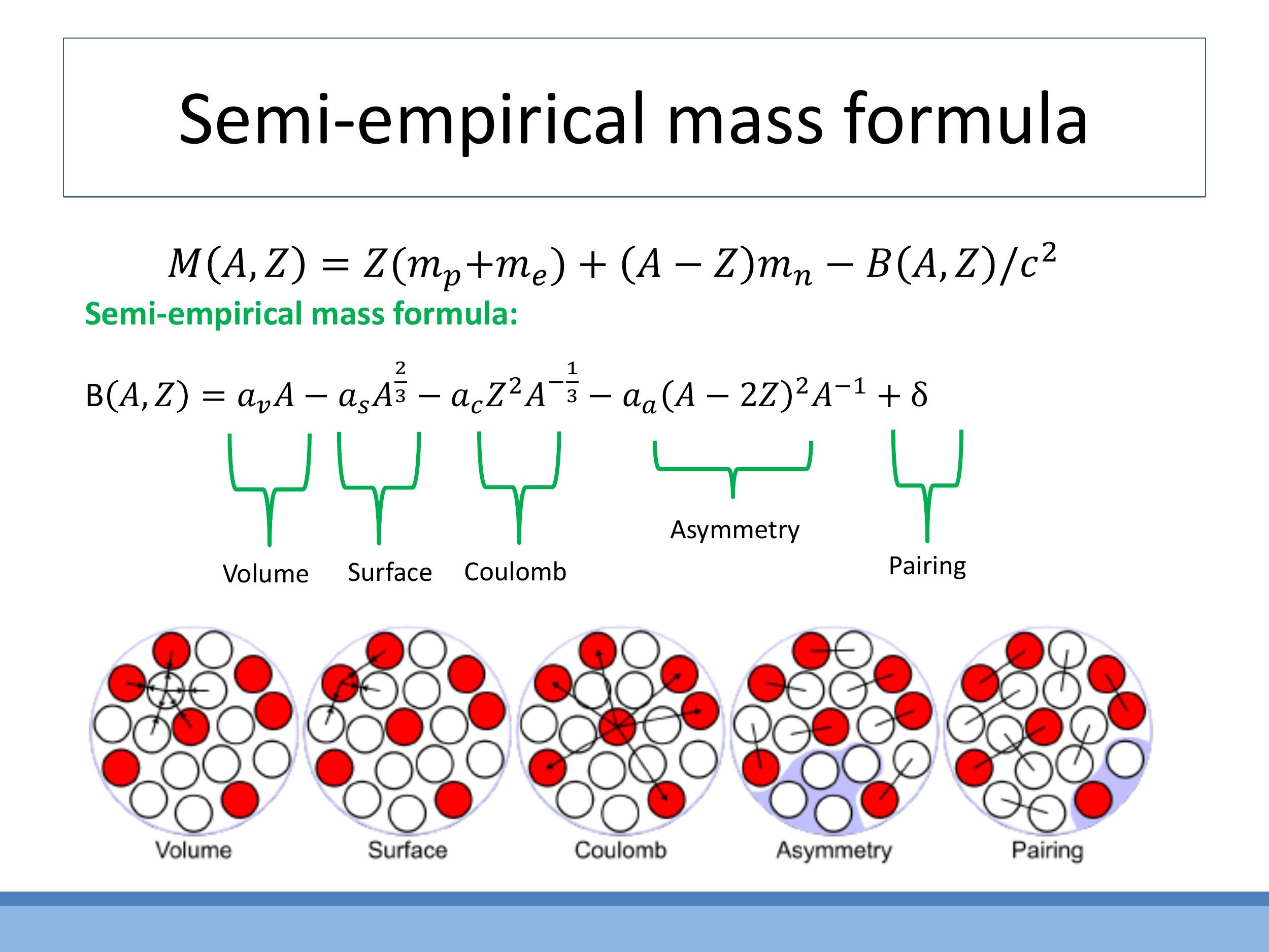
The Semi-empirical Mass Formula (SEMF) is a model used in nuclear physics to approximate the binding energy $B(A, Z)$ of an atomic nucleus, where $A$ is the total number of nucleons (protons and neutrons) and $Z$ is the number of protons. Inspired by the liquid-drop model of the nucleus, it captures various physical effects:
$$
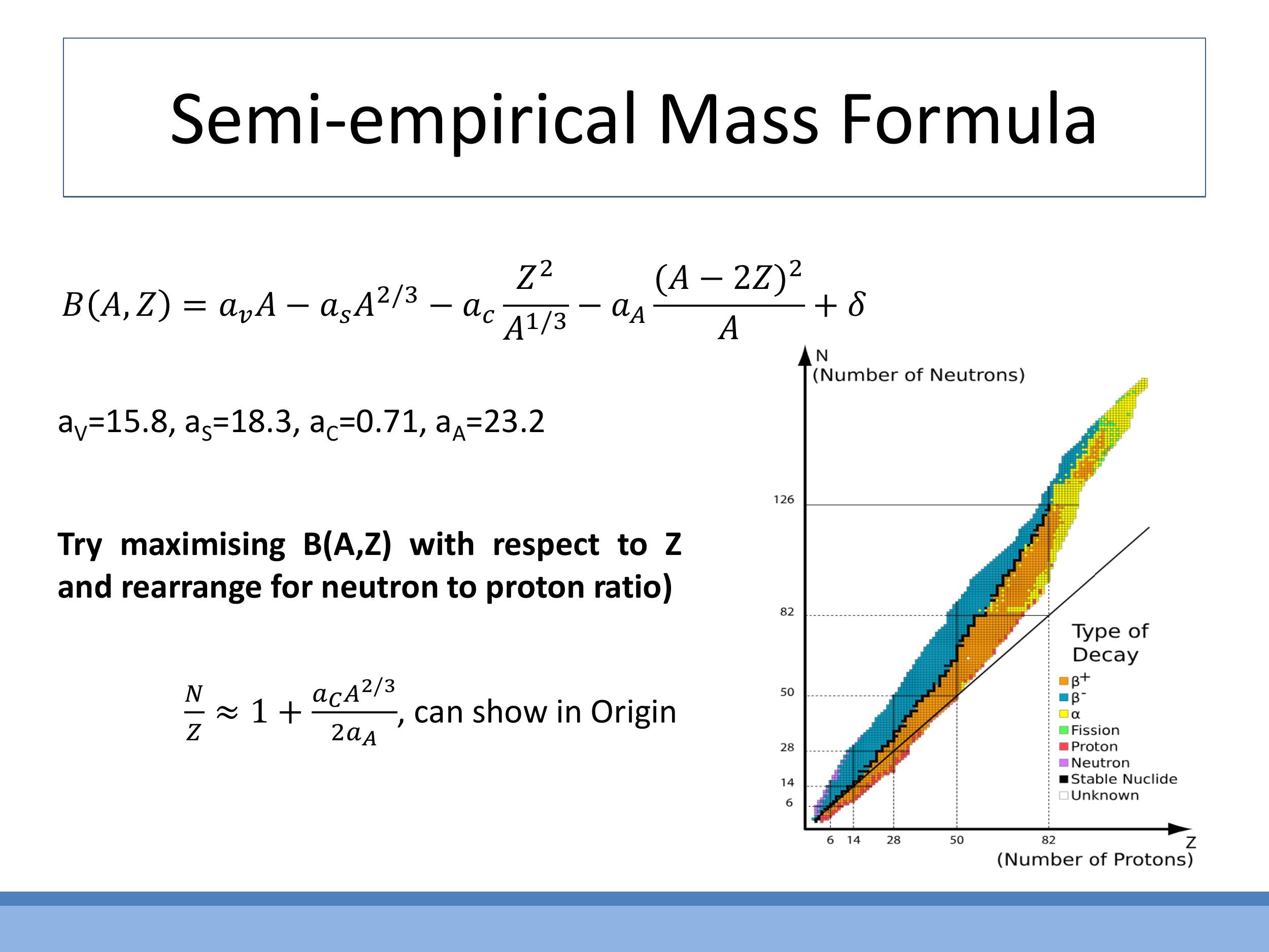
B(A, Z) = a_v A - a_s A^{2/3} - a_c \frac{Z^2}{A^{1/3}} - a_a \frac{(A - 2Z)^2}{A} + \delta
$$
Each term in the formula has a physical interpretation: the $a_v A$ term represents the bulk strong-force binding energy; the $a_s A^{2/3}$ term accounts for reduced binding at the nuclear surface; the $a_c Z^2 / A^{1/3}$ term describes the electrostatic repulsion between protons; the $a_a (A - 2Z)^2 / A$ term penalises imbalances between the number of neutrons and protons; and the $\delta$ term accounts for extra stability due to nucleon pairing.
This formula qualitatively explains the "valley of stability" observed on the nuclide chart, showing how the neutron-to-proton ratio tends to increase with increasing atomic mass $A$. By maximising $B(A, Z)$ with respect to $Z$, one can derive the approximate trend for the neutron-to-proton ratio ($N/Z$) across the periodic table, illustrating the power of such simple models to capture complex physical phenomena.
Key takeaways
Properties of Matter marks a conceptual shift from few-body mechanics to systems involving many particles, where averaging and emergent phenomena are central. Temperature, a quantity we use daily, is a practical example of a many-body average. Collective phenomena, such as ferromagnetism, shape-memory effects, and superconductivity, are real, observable, and driven by the cooperative behaviour of constituent particles or by thermodynamic phase transitions.
The atomic picture has evolved from philosophical ideas to a modern quantum-mechanical view, where electrons occupy probabilistic orbitals around a nucleus of protons and neutrons. Essential quantitative tools for this course include the atomic mass unit ($\text{u}$ or $\text{Da}$), relative atomic mass ($A_r$), the mole, and Avogadro's number ($N_A$). Understanding how isotopic abundances lead to non-integer values for $A_r$ is crucial. A simple packing model can link bulk density and $A_r$ to an estimate of atomic radius, which, despite its approximations, is often "good enough" to provide useful physical insight.
A key cultural aspect of this course is the normalisation of approximations and simple models. These are not second-best solutions but often the right tools for gaining quick physical insight. Finally, some administrative essentials: you must take your own lecture notes, though slides and handwritten derivations will be uploaded. Recommended texts are provided, and attending lectures can offer "easter eggs" that may confer exam advantages.
## Lecture 1: Introduction and ‘Atomos’
### 0) Orientation: How this course works and what to expect


This course, Properties of Matter (PoM), is taught by Dr Ross Springell, an Associate Professor in the School of Physics. While you may be familiar with mechanics, this course shifts focus to understanding systems containing many particles, such as gases, liquids, and solids. Dr Springell's research background is in solid-state and condensed matter physics, particularly with heavy elements like actinides, and includes applications in nuclear fuels, waste, and tritium storage.
Unlike some other courses, pre-written lecture notes will not be provided. You are expected to maintain your own notes during lectures. However, the lecture slides and handwritten derivations shown in class will be uploaded to Blackboard after each session. Each lecture begins with a slide outlining the learning outcomes, which serve as a guide but won't be read out in detail during the lecture itself. The course content has been slightly reduced this year based on previous feedback.
For further reading, several textbooks are recommended: Tipler & Mosca, Blundell & Blundell, and Flowers & Mendoza. G. C. King's "Physics of Matter" is particularly recommended as it aligns closely with the course content, though an eBook version is not currently available. This introductory lecture contains mostly non-examinable material. However, you are expected to be able to perform basic calculations involving atomic masses, moles, and atomic sizes.
> **⚠️ Exam Alert!** The lecturer explicitly stated: "Sometimes I'll give away easter eggs, perhaps as to what might be in the exam... in order to give some advantage, at least to those that turn up to the lectures." This means attending lectures can provide insights into examinable content.
Materials and condensed matter physics is a vast and active research area, offering numerous career opportunities. Students interested in this field can explore summer internships (often for those in their penultimate year), MSc programmes in Nuclear Science & Engineering, or PhD positions. Information on these opportunities is often posted on the third-floor noticeboard.
### 1) From single-particle mechanics to many-body physics

This course represents a significant shift from the classical mechanics you may be used to, which typically deals with a small number of particles or bodies with well-defined initial conditions, such as projectile motion. When dealing with real materials and macroscopic matter, like the air in a room or atoms in a solid, the number of particles is astronomically large. Tracking the individual behaviour of each particle becomes an impossible task due to the sheer number of degrees of freedom involved.
To address this "many-body problem," we adopt new strategies. Instead of focusing on individual particles, we use averaged, emergent quantities to describe the system's collective behaviour. Temperature is a perfect example: we use it daily to describe the average kinetic energy of countless particles without explicitly tracking each one. This approach allows us to understand emergent phenomena, which are complex, large-scale behaviours that arise from the interactions of many individual components and are not predictable from the properties of single constituents alone.
Historically, the scientific trajectory reflects this shift. Early deterministic approaches by figures like Newton and Laplace focused on few-body systems. However, the Industrial Revolution's need to optimise steam engines drove the development of thermodynamics. This led to pioneers like Fourier (heat transfer), Clausius (entropy), Maxwell (molecular speed distributions), Boltzmann (statistical mechanics), and Kelvin (absolute temperature) establishing the tools needed to describe many-body systems.
### 2) Emergence in practice: intuition before equations

Collective behaviour illustrates how many interacting units can produce stable, large-scale patterns that are not predictable by modelling one unit alone. For example, a murmuration of starlings forms intricate, coordinated aerial displays that no computational model of individual birds could foresee. Similarly, ants can cooperate to build living bridges, as shown in the image, where individual ants link together to span gaps. This biological example helps build an intuition for emergence without immediately diving into complex mathematics.
This same principle applies directly to physical materials. The electronic, magnetic, and superconducting properties that we observe in matter arise from the collective behaviour of countless electrons and the atomic-scale interactions between them. Understanding these emergent properties, where the whole is greater than the sum of its parts, is fundamental to the study of the Properties of Matter. This course will focus on building this physical understanding before formalising it with equations.
### 3) Demonstrations of thermodynamic and collective transitions
#### 3.1 Ferromagnetism and the Curie temperature (Nickel + magnet + heat)
We can observe emergent phenomena through simple demonstrations. Consider a piece of nickel, an elemental ferromagnet, attracted to a permanent magnet at room temperature. When the nickel is heated with a flame, it detaches from the magnet. As it cools in the air, it reattaches, creating an oscillation. This happens because ferromagnets are composed of many microscopic magnetic moments that align collectively, leading to a strong attraction. Heating injects thermal energy into the material, which randomises these moments above a specific point called the Curie temperature. Above this temperature, the material transitions from a ferromagnetic (ordered, strongly attractive) state to a paramagnetic (disordered, weakly attractive) state. This is a reversible thermodynamic transition driven by temperature.
#### 3.2 Shape-memory alloys (deform → hot water → original shape)
Another striking example is a shape-memory alloy. If you deform a paperclip made from such an alloy into a random shape, it will instantly return to its original "remembered" form when placed in hot water. This phenomenon is due to a thermodynamic phase transition between two crystal structures. At low temperatures, the alloy exists in a phase that can easily accommodate deformation without breaking atomic bonds; instead, it rearranges internal "twin" structures. When heated, it transitions to a high-temperature cubic phase with a single preferred configuration, forcing it back to the shape it was originally formed in.
#### 3.3 Type II superconductivity and flux pinning (YBCO + magnet + liquid nitrogen)
A dramatic demonstration of collective behaviour is quantum levitation using a Type II superconductor. When a YBCO (Yttrium Barium Copper Oxide) ceramic puck is cooled below its transition temperature (around $92\,\text{K}$) with liquid nitrogen ($77\,\text{K}$), a small magnet placed above it will levitate and become "pinned" in position. This means the magnet is locked and can even be inverted without falling. Superconductors exhibit zero electrical resistance and strong diamagnetism (the Meissner effect), expelling magnetic fields. However, Type II superconductors allow quantised magnetic flux lines to penetrate through discrete, non-superconducting regions. These flux lines become trapped or "pinned" within the material, stabilising the levitation and fixing the magnet's relative position. The discovery of these "high-temperature" superconductors (superconducting above $77\,\text{K}$) was significant because liquid nitrogen is much cheaper than liquid helium. The precise mechanism behind this type of superconductivity is still an active area of research.
### 4) The atomic picture: a brief historical scaffold

Our understanding of the atom has evolved significantly over time. Beginning with the philosophical concept of "atomos" (indivisible particles) from ancient Greek thinkers like Leucippus and Democritus, the modern atomic picture began to take shape with John Dalton's atomic theory in the early $19^\text{th}$ century. This was followed by J. J. Thomson's "plum pudding" model, which posited a positively charged sphere with embedded electrons. Ernest Rutherford's gold foil experiment then revealed the existence of a small, dense, positively charged nucleus, leading to the nuclear atom model. Niels Bohr further refined this with his model of electrons orbiting the nucleus in quantised energy levels.
The modern view of the atom, however, is rooted in quantum mechanics, building on the work of Schrödinger and de Broglie. In this picture, electrons are not tiny particles orbiting a nucleus, but rather wave-like entities that exist in probabilistic orbitals or "clouds" around the nucleus. These orbitals correspond to discrete energy levels. The nucleus itself is composed of protons and neutrons, and its properties are described by nuclear physics. While Bohr's model provides a useful conceptual stepping stone, the wave-mechanical and probabilistic description offers a more accurate representation of electron behaviour.
### 5) Quantitative foundations: mass, moles, and atomic size


#### 5.1 Atomic mass units and isotopes
To quantify matter at the atomic scale, we use the atomic mass unit ($\text{u}$), also known as the Dalton ($\text{Da}$). This unit is precisely defined based on the carbon-12 ($^{12}\text{C}$) atom: one $^{12}\text{C}$ atom has a mass of exactly $12\,\text{u}$. From this, we know that $1\,\text{u} \approx 1.66 \times 10^{-27}\,\text{kg}$. The relative atomic mass ($A_r$) is a unitless quantity that compares the mass of an atom to $1/12^\text{th}$ the mass of a $^{12}\text{C}$ atom:
$$ A_r = \frac{\text{Mass of atom}}{\text{Mass of } ^{12}\text{C atom}} \times 12 $$
The atomic masses listed on the periodic table, such as carbon's $12.011$, are often non-integers. This is because most elements exist naturally as a mixture of different isotopes, which are atoms with the same number of protons but different numbers of neutrons. The listed atomic mass is a weighted average of the masses of these isotopes, taking into account their natural abundance. For example, carbon's $12.011$ reflects the natural abundance of $^{12}\text{C}$ and $^{13}\text{C}$.
#### 5.2 Counting particles: the mole and Avogadro’s number
When dealing with macroscopic quantities of matter, we use the mole ($\text{mol}$) to count particles. One mole is defined as the amount of substance that contains as many elementary entities (atoms, molecules, etc.) as there are atoms in exactly $12\,\text{g}$ of $^{12}\text{C}$. This definition directly leads to Avogadro's number ($N_A$), which is the number of entities in one mole:
$$ N_A = \frac{0.012\,\text{kg}}{\text{mass of one } ^{12}\text{C atom}} \approx 6.022 \times 10^{23}\,\text{mol}^{-1} $$
Avogadro's number is crucial because it provides a link between macroscopic quantities that we can measure (like grams or cubic centimetres) and the microscopic count of atoms or molecules.
#### 5.3 Estimating how big an atom is (simple cubic packing model)
We can estimate the size of an atom using a simple "back-of-the-envelope" calculation, which is often surprisingly effective. In this model, we treat atoms as hard spheres of radius $R$ and assume they are packed in a simple cubic lattice. In this arrangement, each atom effectively occupies a cubic volume with side length $2R$, so the volume per atom is $(2R)^3$.
To connect this microscopic picture to macroscopic data, we can calculate the molar volume ($V_m$) from a substance's relative atomic mass ($A_r$, in $\text{g}\,\text{mol}^{-1}$) and its bulk density ($\rho$, in $\text{g}\,\text{cm}^{-3}$): $V_m = A_r / \rho$. We also know that the molar volume is approximately the volume per atom multiplied by Avogadro's number: $V_m \approx N_A (2R)^3$. Equating these two expressions for molar volume allows us to solve for the atomic radius $R$:
$$ R \approx \frac{1}{2} \left( \frac{A_r}{\rho N_A} \right)^{1/3} $$
As an example, let's estimate the radius of a uranium atom. Given its relative atomic mass $A_r = 238\,\text{g}\,\text{mol}^{-1}$ and density $\rho = 19\,\text{g}\,\text{cm}^{-3}$, the formula yields an atomic radius of $R \approx 1.38\,\text{Å}$ (or $0.138\,\text{nm}$). This crude model provides a result remarkably close to experimental values, which are typically around $1.75\,\text{Å}$, demonstrating the power and utility of such approximate models in physics. Being comfortable with these kinds of estimations and back-of-the-envelope reasoning is a valuable skill in this course.
### 6) The modelling mindset: “close enough” is often powerful

In physics, it's not always necessary to have exact microscopic detail to solve a problem. Often, a well-chosen, simplified model, coupled with reasonable approximations, can produce incredibly useful and testable estimates. This "close enough" approach allows us to gain quick physical insight and is a core problem-solving strategy in Properties of Matter. Throughout this course, we will frequently link macroscopic observables to microscopic models with simplifying assumptions, then sanity-check our results against experimental data. This iterative process of estimation, comparison, and refinement is fundamental to scientific discovery.
## Appendix: Semi-empirical Mass Formula (SEMF)


*Side Note:* This material is supplementary and won't be examined, but provides useful context.
The Semi-empirical Mass Formula (SEMF) is a model used in nuclear physics to approximate the binding energy $B(A, Z)$ of an atomic nucleus, where $A$ is the total number of nucleons (protons and neutrons) and $Z$ is the number of protons. Inspired by the liquid-drop model of the nucleus, it captures various physical effects:
$$ B(A, Z) = a_v A - a_s A^{2/3} - a_c \frac{Z^2}{A^{1/3}} - a_a \frac{(A - 2Z)^2}{A} + \delta $$
Each term in the formula has a physical interpretation: the $a_v A$ term represents the bulk strong-force binding energy; the $a_s A^{2/3}$ term accounts for reduced binding at the nuclear surface; the $a_c Z^2 / A^{1/3}$ term describes the electrostatic repulsion between protons; the $a_a (A - 2Z)^2 / A$ term penalises imbalances between the number of neutrons and protons; and the $\delta$ term accounts for extra stability due to nucleon pairing.
This formula qualitatively explains the "valley of stability" observed on the nuclide chart, showing how the neutron-to-proton ratio tends to increase with increasing atomic mass $A$. By maximising $B(A, Z)$ with respect to $Z$, one can derive the approximate trend for the neutron-to-proton ratio ($N/Z$) across the periodic table, illustrating the power of such simple models to capture complex physical phenomena.
## Key takeaways
Properties of Matter marks a conceptual shift from few-body mechanics to systems involving many particles, where averaging and emergent phenomena are central. Temperature, a quantity we use daily, is a practical example of a many-body average. Collective phenomena, such as ferromagnetism, shape-memory effects, and superconductivity, are real, observable, and driven by the cooperative behaviour of constituent particles or by thermodynamic phase transitions.
The atomic picture has evolved from philosophical ideas to a modern quantum-mechanical view, where electrons occupy probabilistic orbitals around a nucleus of protons and neutrons. Essential quantitative tools for this course include the atomic mass unit ($\text{u}$ or $\text{Da}$), relative atomic mass ($A_r$), the mole, and Avogadro's number ($N_A$). Understanding how isotopic abundances lead to non-integer values for $A_r$ is crucial. A simple packing model can link bulk density and $A_r$ to an estimate of atomic radius, which, despite its approximations, is often "good enough" to provide useful physical insight.
A key cultural aspect of this course is the normalisation of approximations and simple models. These are not second-best solutions but often the right tools for gaining quick physical insight. Finally, some administrative essentials: you must take your own lecture notes, though slides and handwritten derivations will be uploaded. Recommended texts are provided, and attending lectures can offer "easter eggs" that may confer exam advantages.