Lecture 6: Maxwell-Boltzmann Distribution (Thermal energy in gases, part 3)
0) Orientation, learning outcomes, and admin
This lecture focuses on deriving the Maxwell-Boltzmann (MB) distributions, starting from Boltzmann's statistical weight in one dimension (velocity components) and extending to two and three-dimensional speeds. The goal is to connect these distributions to average quantities, such as mean square speeds and average kinetic energies, and to the equipartition theorem. By the end of this lecture, a student should be able to derive the Maxwell-Boltzmann distribution in one, two, and three dimensions, including its normalisation. Furthermore, they should be able to calculate average speeds and average kinetic energies directly from these distributions and relate their findings to the equipartition theorem, specifically the principle of $\frac{1}{2}kT$ energy per quadratic degree of freedom.
Lecture recordings are available via the "Replay" section on Blackboard. A problems class will be held to work through selected derivations and examples from this lecture.
⚠️ Exam Alert! The lecturer explicitly stated: "I recommend you definitely come to the problems class tomorrow." Students should attend to gain practice with the derivations and calculations that are relevant for assessment.
1) Recap: Boltzmann factor and extreme-temperature limits
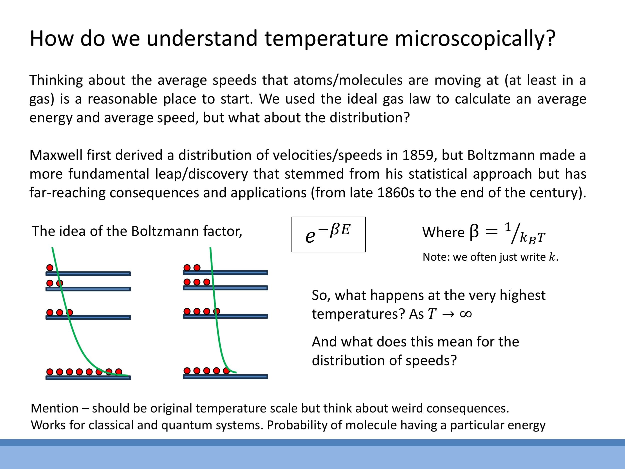
The Boltzmann factor, $e^{-\beta E}$, where $\beta = \frac{1}{kT}$, quantifies the statistical weight of a state with energy $E$ at a given temperature $T$. This factor describes how populations of particles are distributed across different energy levels. At higher temperatures, particles are more likely to occupy higher energy states.
In the high-temperature limit, as $T \rightarrow \infty$, the term $\beta$ approaches zero. Consequently, the Boltzmann factor $e^{-\beta E}$ approaches $e^0 = 1$. Physically, this means that at infinitely high temperatures, all energy levels become equally populated. This provides an intuitive understanding of how increasing thermal energy tends to homogenise the distribution of particles across available states.
Side Note: In unusual, non-equilibrium conditions, it is possible for higher energy levels to be more populated than lower ones, a phenomenon known as population inversion. Mathematically, this would imply a negative absolute temperature. Such states are realised in devices like lasers and are considered "hotter" than infinite temperature in terms of their energy flow characteristics. However, all thermodynamic systems considered in this course will operate at normal, positive absolute temperatures.
2) From microstate weights to a probability density
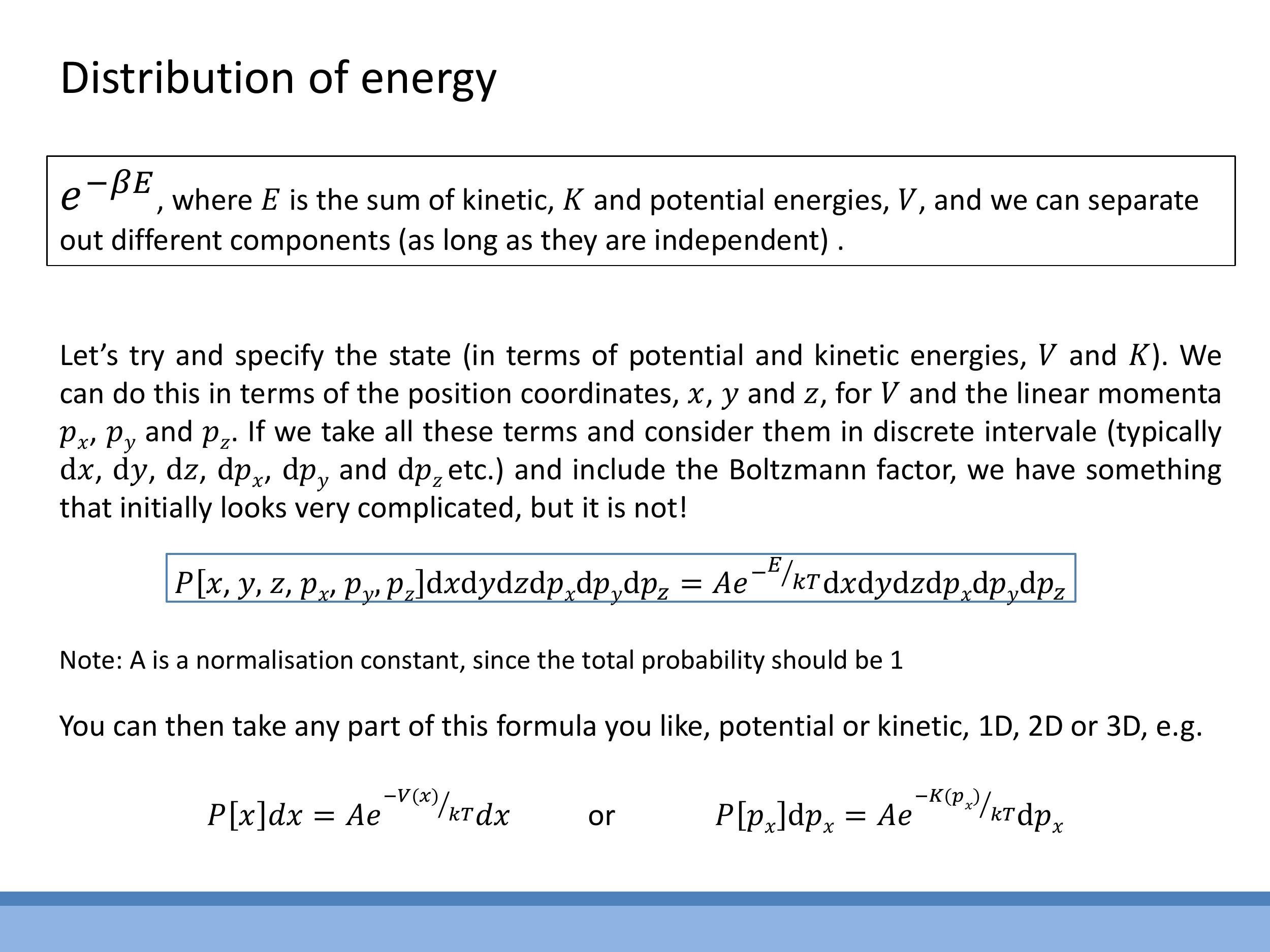
The probability of a system being in a specific microstate, defined by its position $(x, y, z)$ and momentum $(p_x, p_y, p_z)$, is given by the expression:
$$
P[x, y, z, p_x, p_y, p_z] \, dx \, dy \, dz \, dp_x \, dp_y \, dp_z = A e^{-E / kT} \, dx \, dy \, dz \, dp_x \, dp_y \, dp_z
$$
Here, $A$ is a normalisation constant, ensuring that the total probability of the particle being in any possible state (i.e., integrated over all possible positions and momenta) sums to 1. The total energy $E$ includes both kinetic and potential energy components.
A key property of this probability density is its separability. If the energy components are independent, the distribution can be simplified to consider only a subset of variables, such as a single momentum component. This allows for the initial derivation of one-dimensional velocity-component distributions, which then serves as a foundation for understanding more complex speed distributions in two and three dimensions.
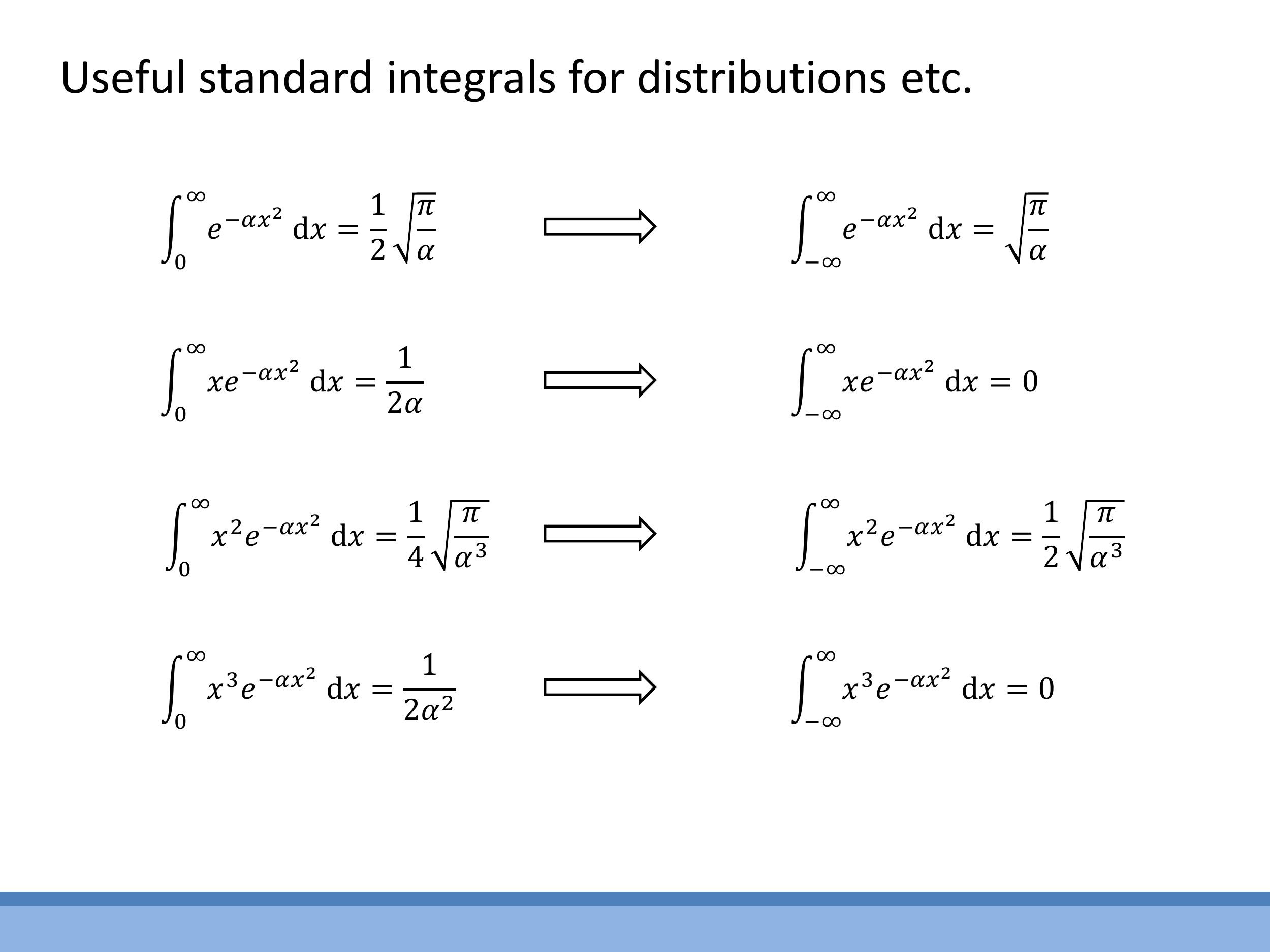
The derivation of these distributions often requires the use of standard Gaussian integrals. These integral forms will be provided in examinations and will be thoroughly worked through during the problems class, so memorisation is not required.
3) 1D velocity-component distribution: derivation and averages
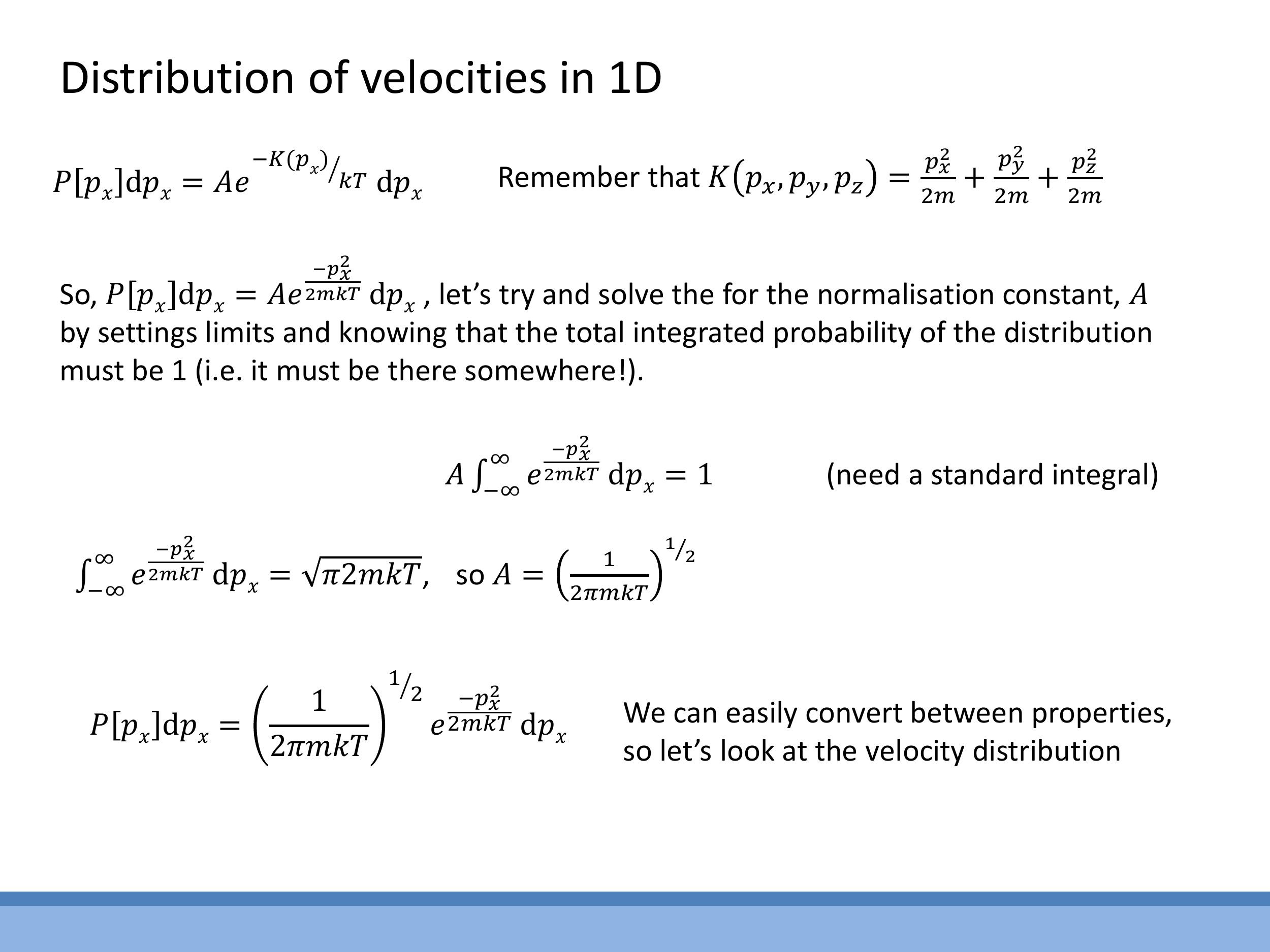
To derive the probability distribution for a single velocity component, $P[v_x]$, one starts with the probability distribution for momentum $P[p_x]$, where the kinetic energy is $K = \frac{p_x^2}{2m}$.
$$
P[p_x] dp_x = A e^{-\frac{p_x^2}{2mkT}} dp_x
$$
The normalisation constant $A$ is determined by integrating this expression over all possible momenta (from $-\infty$ to $+\infty$) and setting the total probability to 1. Using the standard integral $\int_{-\infty}^{\infty} e^{-\alpha x^2} dx = \sqrt{\frac{\pi}{\alpha}}$, with $\alpha = \frac{1}{2mkT}$, the normalisation constant is found to be $A = \left( \frac{1}{2\pi mkT} \right)^{1/2}$.
The distribution is then converted from momentum $p_x$ to velocity $v_x$ using the relationships $p_x = mv_x$ and $dp_x = m dv_x$.
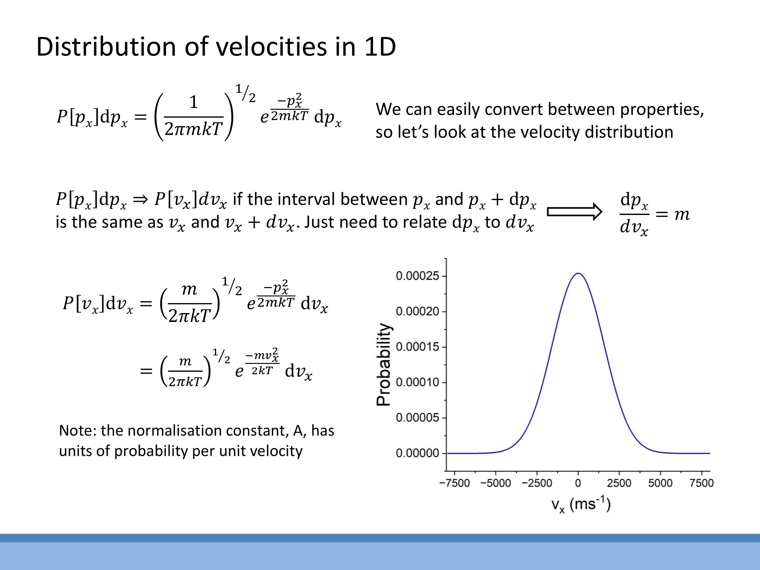
This yields the normalised one-dimensional velocity distribution:
$$
P[v_x] dv_x = \left( \frac{m}{2 \pi k T} \right)^{1/2} e^{- \frac{m v_x^2}{2 k T}} dv_x
$$
This distribution is a symmetric Gaussian curve centered at $v_x = 0$. Due to its symmetry, the average velocity $\overline{v_x}$ is zero.
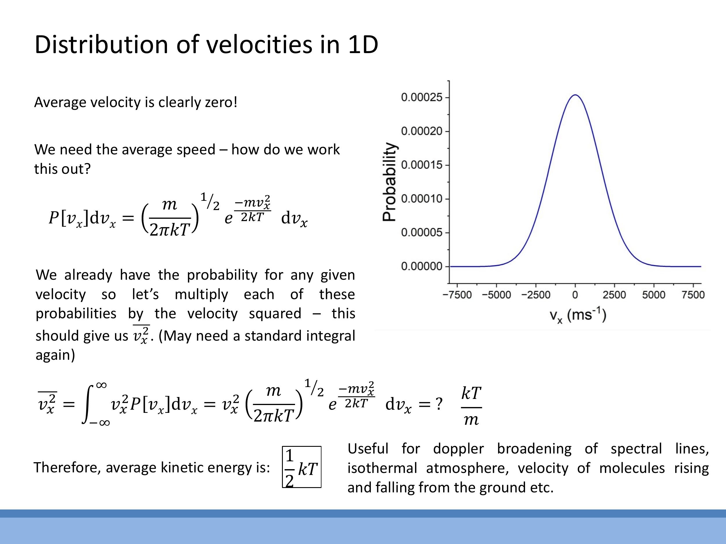
To obtain a meaningful measure of speed, the mean square velocity $\overline{v_x^2}$ is calculated by integrating $v_x^2$ weighted by the probability distribution $P[v_x]$ over all velocities. Using the appropriate standard integral, the result is:
$$
\overline{v_x^2} = \frac{kT}{m}
$$
From this, the average kinetic energy per degree of freedom (in one dimension) is:
$$
\frac{1}{2} m \overline{v_x^2} = \frac{1}{2} m \left( \frac{kT}{m} \right) = \frac{1}{2} kT
$$
This result perfectly aligns with the equipartition theorem, which states that each quadratic degree of freedom contributes an average energy of $\frac{1}{2}kT$. This one-dimensional component distribution is fundamental for understanding phenomena such as Doppler broadening of spectral lines and models of isothermal atmospheres.
4) Why speed distributions differ from component Gaussians: state counting
The Maxwell-Boltzmann distribution for molecular speeds in two and three dimensions differs significantly from the simple Gaussian distribution for velocity components
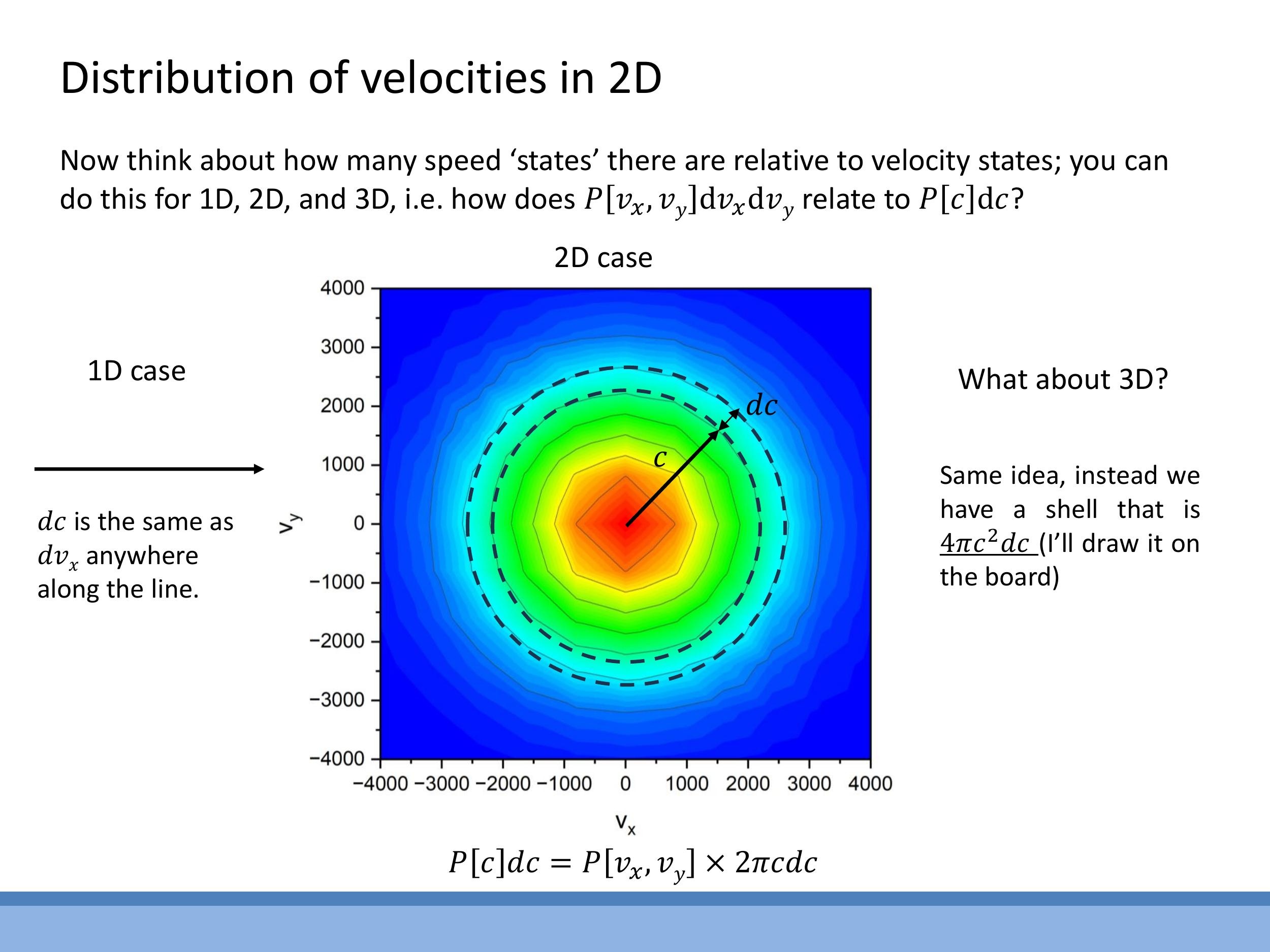
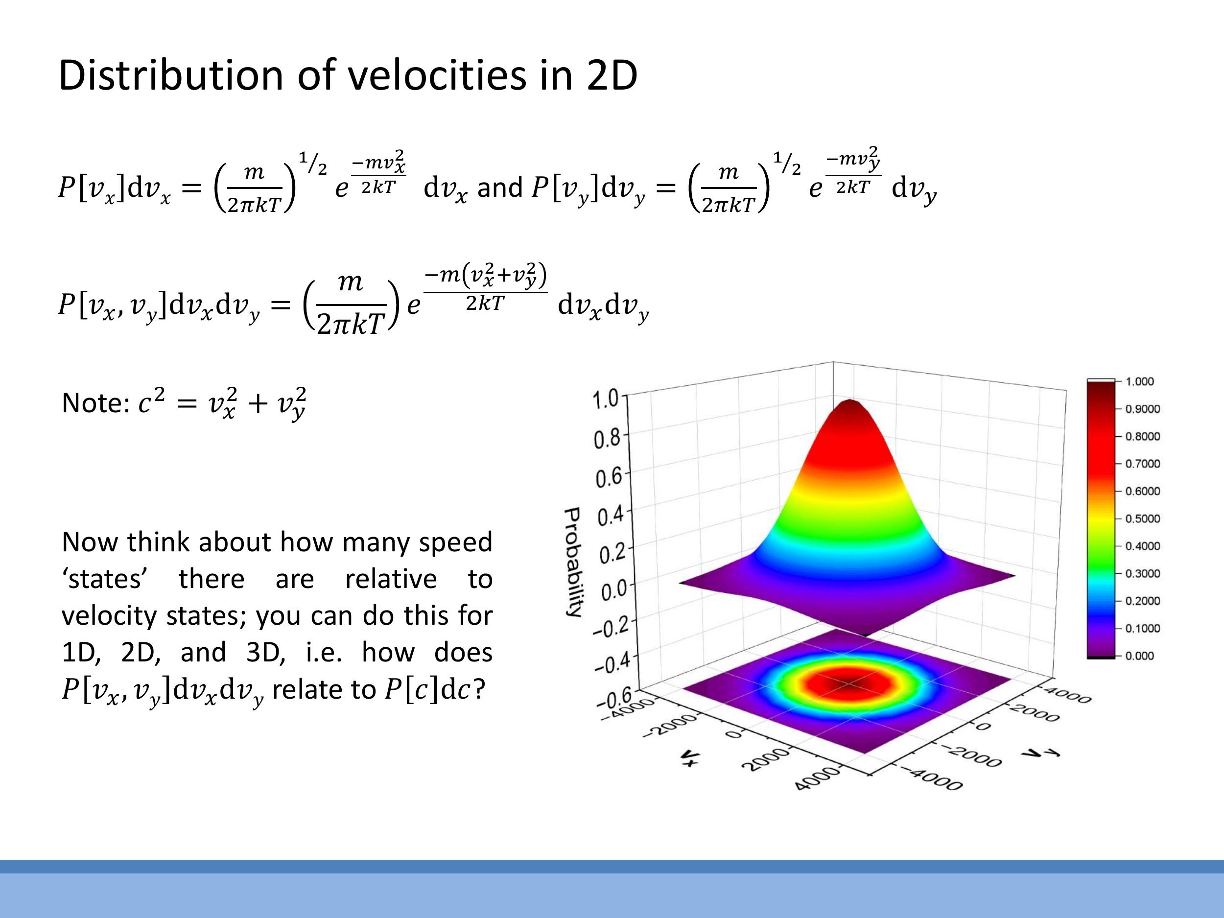
In two dimensions, all velocity vectors $(v_x, v_y)$ that correspond to a given speed $c$ lie on a circle of radius $c$ in velocity space. The number of states within a small speed interval $[c, c+dc]$ is proportional to the circumference of this circle, $2\pi c \, dc$.
In three dimensions, the velocity states for a given speed $c$ lie on the surface of a sphere of radius $c$. The number of states in the interval $[c, c+dc]$ is proportional to the surface area of this sphere, $4\pi c^2 \, dc$.
Consequently, the speed distributions in 2D and 3D are products of the exponential Boltzmann factor, $e^{-mc^2/2kT}$, and this state-counting factor ($c$ in 2D, $c^2$ in 3D). This results in a characteristic shape that begins at zero, rises to a peak at an intermediate speed, and then decays exponentially, unlike the symmetric Gaussian for velocity components.
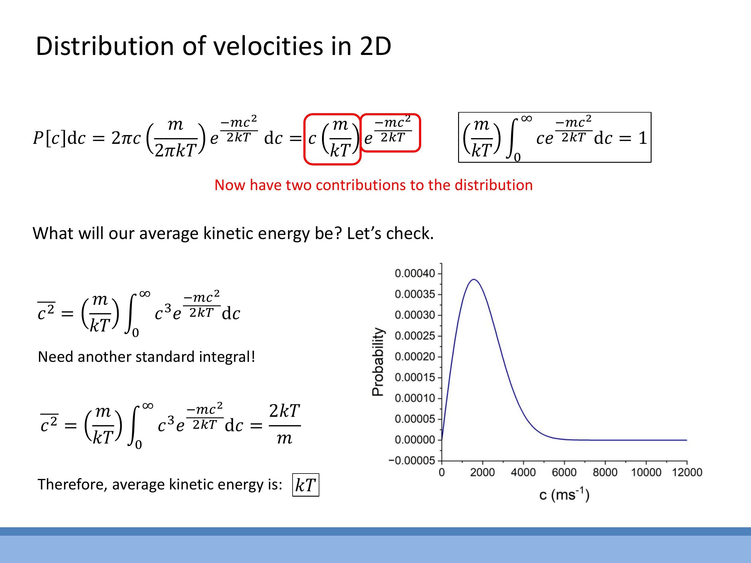
Combining the Boltzmann factor with the two-dimensional state-counting factor ($2\pi c \, dc$) and applying normalisation yields the 2D Maxwell-Boltzmann speed distribution:
$$
P[c]dc = c \frac{m}{kT} e^{-mc^2 / 2kT} dc
$$
To determine the average kinetic energy in two dimensions, the mean square speed $\overline{c^2}$ is calculated by integrating $c^2$ weighted by this distribution. Using the relevant standard integral for the $c^3$ -term, the result is:
$$
\overline{c^2} = \frac{2kT}{m}
$$
Therefore, the average kinetic energy in two dimensions is $\frac{1}{2} m \overline{c^2} = \frac{1}{2} m \left( \frac{2kT}{m} \right) = kT$. This result, $kT$, is consistent with the equipartition theorem, as there are two quadratic degrees of freedom for translational motion in two dimensions, each contributing $\frac{1}{2}kT$. The shape of the distribution, rising from zero at small $c$ and then falling, is a direct consequence of the linear increase in available states with $c$ competing with the exponential decay of the Boltzmann factor.
6) 3D Maxwell-Boltzmann speed distribution: full form and anatomy
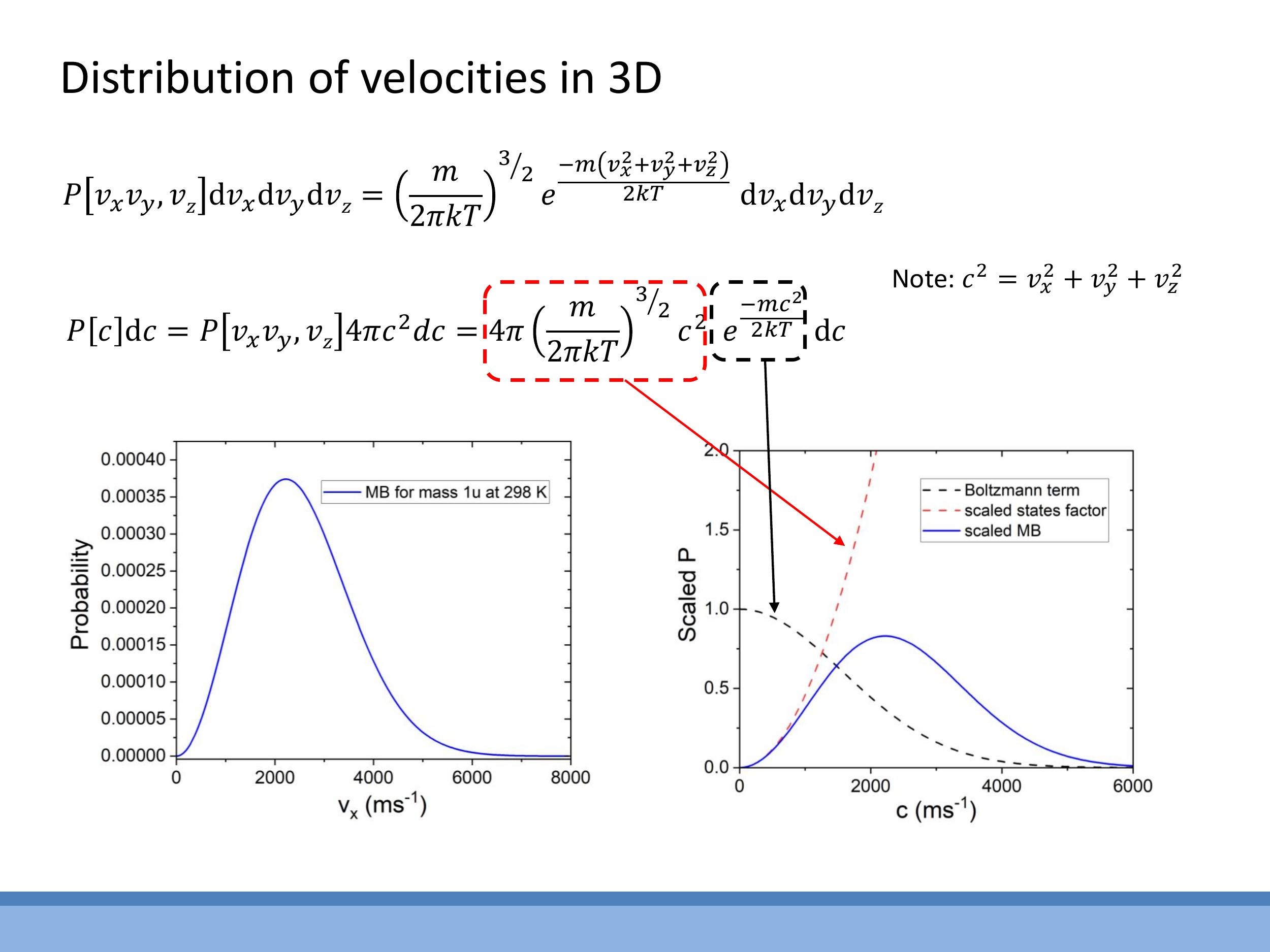
The starting point for the 3D speed distribution is the joint probability distribution for the three velocity components $v_x, v_y, v_z$:
$$
P[v_x v_y v_z] \, dv_x dv_y dv_z = \left( \frac{m}{2 \pi k T} \right)^{3/2} e^{\frac{-m(v_x^2 + v_y^2 + v_z^2)}{2kT}} dv_x dv_y dv_z
$$
To convert this to a distribution of speeds $c$, where $c^2 = v_x^2 + v_y^2 + v_z^2$, the three-dimensional state-counting factor of $4\pi c^2 \, dc$ is introduced. This factor accounts for the increasing number of velocity states as speed increases. The resulting full 3D Maxwell-Boltzmann speed distribution is:
$$
P[c] \, dc = 4 \pi \left( \frac{m}{2 \pi k T} \right)^{3/2} c^2 e^{- \frac{m c^2}{2 k T}} \, dc
$$
The characteristic shape of this distribution is a product of two competing terms: the $c^2$ factor, which increases quadratically with speed and pushes the probability up at small $c$, and the exponential Boltzmann term, $e^{-mc^2/2kT}$, which causes the distribution to decay rapidly at large $c$. The combination of these two factors results in the familiar bell-shaped curve that starts at zero, rises to a peak (representing the most probable speed), and then gradually tails off. This distribution specifically describes the speeds of particles, not their individual velocity components.
7) What was deferred and what comes next
In this lecture, the conceptual construction of the Maxwell-Boltzmann distributions was emphasised, with the full one-dimensional derivation completed in detail. For the two and three-dimensional distributions, the normalisation procedures and the use of standard integrals were outlined, and the final results presented.
The upcoming problems class will provide an opportunity to work through a full example that utilises these distributions and the necessary standard integrals. Students are encouraged to bring any questions they may have regarding normalisation techniques and the calculation of average values from these distributions for further clarification and practice.
Key takeaways
The Boltzmann factor, $e^{-E/kT}$, dictates the population of energy levels; as $T \rightarrow \infty$, all levels become equally populated. Population inversion, which implies negative absolute temperature, is a non-equilibrium state found in devices like lasers, but this course strictly deals with positive temperatures.
Derived from $P \propto e^{-E/kT}$, the one-dimensional velocity component distribution is a Gaussian: $P(v_x) = \left( \frac{m}{2\pi kT} \right)^{1/2} e^{-m v_x^2/2kT}$. Its average velocity is zero, and the mean square velocity is $\overline{v_x^2} = \frac{kT}{m}$. This leads to an average kinetic energy per component of $\frac{1}{2}kT$, validating the equipartition theorem for a single quadratic degree of freedom.
Speed distributions differ from component Gaussians due to "state counting," which accounts for the increasing number of velocity combinations that yield the same speed:
- In two dimensions, $P(c) \propto c \, e^{-mc^2/2kT} $, and the average kinetic energy is $ kT $, consistent with two degrees of freedom each contributing $ \frac{1}{2}kT$.
- In three dimensions, the full Maxwell-Boltzmann speed distribution is $P(c) \, dc = 4\pi \left( \frac{m}{2\pi kT} \right)^{3/2} c^2 e^{-mc^2/2kT} \, dc$.
The shape of the Maxwell-Boltzmann speed distributions is a product of a geometrically increasing states factor ($c$ or $c^2$) and a decaying Boltzmann exponential term, resulting in a characteristic peak at intermediate speeds. Standard Gaussian integrals are essential for normalisation and calculating average values; these will be provided in exams and practised in problems classes.
## Lecture 6: Maxwell-Boltzmann Distribution (Thermal energy in gases, part 3)
### 0) Orientation, learning outcomes, and admin

This lecture focuses on deriving the Maxwell-Boltzmann (MB) distributions, starting from Boltzmann's statistical weight in one dimension (velocity components) and extending to two and three-dimensional speeds. The goal is to connect these distributions to average quantities, such as mean square speeds and average kinetic energies, and to the equipartition theorem. By the end of this lecture, a student should be able to derive the Maxwell-Boltzmann distribution in one, two, and three dimensions, including its normalisation. Furthermore, they should be able to calculate average speeds and average kinetic energies directly from these distributions and relate their findings to the equipartition theorem, specifically the principle of $\frac{1}{2}kT$ energy per quadratic degree of freedom.
Lecture recordings are available via the "Replay" section on Blackboard. A problems class will be held to work through selected derivations and examples from this lecture.
> **⚠️ Exam Alert!** The lecturer explicitly stated: "I recommend you definitely come to the problems class tomorrow." Students should attend to gain practice with the derivations and calculations that are relevant for assessment.
### 1) Recap: Boltzmann factor and extreme-temperature limits

The Boltzmann factor, $e^{-\beta E}$, where $\beta = \frac{1}{kT}$, quantifies the statistical weight of a state with energy $E$ at a given temperature $T$. This factor describes how populations of particles are distributed across different energy levels. At higher temperatures, particles are more likely to occupy higher energy states.
In the high-temperature limit, as $T \rightarrow \infty$, the term $\beta$ approaches zero. Consequently, the Boltzmann factor $e^{-\beta E}$ approaches $e^0 = 1$. Physically, this means that at infinitely high temperatures, all energy levels become equally populated. This provides an intuitive understanding of how increasing thermal energy tends to homogenise the distribution of particles across available states.
*Side Note:* In unusual, non-equilibrium conditions, it is possible for higher energy levels to be more populated than lower ones, a phenomenon known as population inversion. Mathematically, this would imply a negative absolute temperature. Such states are realised in devices like lasers and are considered "hotter" than infinite temperature in terms of their energy flow characteristics. However, all thermodynamic systems considered in this course will operate at normal, positive absolute temperatures.
### 2) From microstate weights to a probability density

The probability of a system being in a specific microstate, defined by its position $(x, y, z)$ and momentum $(p_x, p_y, p_z)$, is given by the expression:
$$ P[x, y, z, p_x, p_y, p_z] \, dx \, dy \, dz \, dp_x \, dp_y \, dp_z = A e^{-E / kT} \, dx \, dy \, dz \, dp_x \, dp_y \, dp_z $$
Here, $A$ is a normalisation constant, ensuring that the total probability of the particle being in any possible state (i.e., integrated over all possible positions and momenta) sums to 1. The total energy $E$ includes both kinetic and potential energy components.
A key property of this probability density is its separability. If the energy components are independent, the distribution can be simplified to consider only a subset of variables, such as a single momentum component. This allows for the initial derivation of one-dimensional velocity-component distributions, which then serves as a foundation for understanding more complex speed distributions in two and three dimensions.

The derivation of these distributions often requires the use of standard Gaussian integrals. These integral forms will be provided in examinations and will be thoroughly worked through during the problems class, so memorisation is not required.
### 3) 1D velocity-component distribution: derivation and averages

To derive the probability distribution for a single velocity component, $P[v_x]$, one starts with the probability distribution for momentum $P[p_x]$, where the kinetic energy is $K = \frac{p_x^2}{2m}$.
$$ P[p_x] dp_x = A e^{-\frac{p_x^2}{2mkT}} dp_x $$
The normalisation constant $A$ is determined by integrating this expression over all possible momenta (from $-\infty$ to $+\infty$) and setting the total probability to 1. Using the standard integral $\int_{-\infty}^{\infty} e^{-\alpha x^2} dx = \sqrt{\frac{\pi}{\alpha}}$, with $\alpha = \frac{1}{2mkT}$, the normalisation constant is found to be $A = \left( \frac{1}{2\pi mkT} \right)^{1/2}$.
The distribution is then converted from momentum $p_x$ to velocity $v_x$ using the relationships $p_x = mv_x$ and $dp_x = m dv_x$.

This yields the normalised one-dimensional velocity distribution:
$$ P[v_x] dv_x = \left( \frac{m}{2 \pi k T} \right)^{1/2} e^{- \frac{m v_x^2}{2 k T}} dv_x $$
This distribution is a symmetric Gaussian curve centered at $v_x = 0$. Due to its symmetry, the average velocity $\overline{v_x}$ is zero.

To obtain a meaningful measure of speed, the mean square velocity $\overline{v_x^2}$ is calculated by integrating $v_x^2$ weighted by the probability distribution $P[v_x]$ over all velocities. Using the appropriate standard integral, the result is:
$$ \overline{v_x^2} = \frac{kT}{m} $$
From this, the average kinetic energy per degree of freedom (in one dimension) is:
$$ \frac{1}{2} m \overline{v_x^2} = \frac{1}{2} m \left( \frac{kT}{m} \right) = \frac{1}{2} kT $$
This result perfectly aligns with the equipartition theorem, which states that each quadratic degree of freedom contributes an average energy of $\frac{1}{2}kT$. This one-dimensional component distribution is fundamental for understanding phenomena such as Doppler broadening of spectral lines and models of isothermal atmospheres.
### 4) Why speed distributions differ from component Gaussians: state counting

The Maxwell-Boltzmann distribution for molecular *speeds* in two and three dimensions differs significantly from the simple Gaussian distribution for velocity *components*. This difference arises because many combinations of velocity components (e.g., $v_x, v_y, v_z$) can result in the same overall speed $c = \sqrt{v_x^2 + v_y^2 + v_z^2}$. The number of available "speed states" increases with $c$ due to geometric considerations in velocity space.

In two dimensions, all velocity vectors $(v_x, v_y)$ that correspond to a given speed $c$ lie on a circle of radius $c$ in velocity space. The number of states within a small speed interval $[c, c+dc]$ is proportional to the circumference of this circle, $2\pi c \, dc$.
In three dimensions, the velocity states for a given speed $c$ lie on the surface of a sphere of radius $c$. The number of states in the interval $[c, c+dc]$ is proportional to the surface area of this sphere, $4\pi c^2 \, dc$.
Consequently, the speed distributions in 2D and 3D are products of the exponential Boltzmann factor, $e^{-mc^2/2kT}$, and this state-counting factor ($c$ in 2D, $c^2$ in 3D). This results in a characteristic shape that begins at zero, rises to a peak at an intermediate speed, and then decays exponentially, unlike the symmetric Gaussian for velocity components.
### 5) 2D speed distribution: form and average kinetic energy

Combining the Boltzmann factor with the two-dimensional state-counting factor ($2\pi c \, dc$) and applying normalisation yields the 2D Maxwell-Boltzmann speed distribution:
$$ P[c]dc = c \frac{m}{kT} e^{-mc^2 / 2kT} dc $$
To determine the average kinetic energy in two dimensions, the mean square speed $\overline{c^2}$ is calculated by integrating $c^2$ weighted by this distribution. Using the relevant standard integral for the $c^3$-term, the result is:
$$ \overline{c^2} = \frac{2kT}{m} $$
Therefore, the average kinetic energy in two dimensions is $\frac{1}{2} m \overline{c^2} = \frac{1}{2} m \left( \frac{2kT}{m} \right) = kT$. This result, $kT$, is consistent with the equipartition theorem, as there are two quadratic degrees of freedom for translational motion in two dimensions, each contributing $\frac{1}{2}kT$. The shape of the distribution, rising from zero at small $c$ and then falling, is a direct consequence of the linear increase in available states with $c$ competing with the exponential decay of the Boltzmann factor.
### 6) 3D Maxwell-Boltzmann speed distribution: full form and anatomy

The starting point for the 3D speed distribution is the joint probability distribution for the three velocity components $v_x, v_y, v_z$:
$$ P[v_x v_y v_z] \, dv_x dv_y dv_z = \left( \frac{m}{2 \pi k T} \right)^{3/2} e^{\frac{-m(v_x^2 + v_y^2 + v_z^2)}{2kT}} dv_x dv_y dv_z $$
To convert this to a distribution of speeds $c$, where $c^2 = v_x^2 + v_y^2 + v_z^2$, the three-dimensional state-counting factor of $4\pi c^2 \, dc$ is introduced. This factor accounts for the increasing number of velocity states as speed increases. The resulting full 3D Maxwell-Boltzmann speed distribution is:
$$ P[c] \, dc = 4 \pi \left( \frac{m}{2 \pi k T} \right)^{3/2} c^2 e^{- \frac{m c^2}{2 k T}} \, dc $$
The characteristic shape of this distribution is a product of two competing terms: the $c^2$ factor, which increases quadratically with speed and pushes the probability up at small $c$, and the exponential Boltzmann term, $e^{-mc^2/2kT}$, which causes the distribution to decay rapidly at large $c$. The combination of these two factors results in the familiar bell-shaped curve that starts at zero, rises to a peak (representing the most probable speed), and then gradually tails off. This distribution specifically describes the speeds of particles, not their individual velocity components.
### 7) What was deferred and what comes next
In this lecture, the conceptual construction of the Maxwell-Boltzmann distributions was emphasised, with the full one-dimensional derivation completed in detail. For the two and three-dimensional distributions, the normalisation procedures and the use of standard integrals were outlined, and the final results presented.
The upcoming problems class will provide an opportunity to work through a full example that utilises these distributions and the necessary standard integrals. Students are encouraged to bring any questions they may have regarding normalisation techniques and the calculation of average values from these distributions for further clarification and practice.
## Key takeaways
The Boltzmann factor, $e^{-E/kT}$, dictates the population of energy levels; as $T \rightarrow \infty$, all levels become equally populated. Population inversion, which implies negative absolute temperature, is a non-equilibrium state found in devices like lasers, but this course strictly deals with positive temperatures.
Derived from $P \propto e^{-E/kT}$, the one-dimensional velocity component distribution is a Gaussian: $P(v_x) = \left( \frac{m}{2\pi kT} \right)^{1/2} e^{-m v_x^2/2kT}$. Its average velocity is zero, and the mean square velocity is $\overline{v_x^2} = \frac{kT}{m}$. This leads to an average kinetic energy per component of $\frac{1}{2}kT$, validating the equipartition theorem for a single quadratic degree of freedom.
Speed distributions differ from component Gaussians due to "state counting," which accounts for the increasing number of velocity combinations that yield the same speed:
- In two dimensions, $P(c) \propto c \, e^{-mc^2/2kT}$, and the average kinetic energy is $kT$, consistent with two degrees of freedom each contributing $\frac{1}{2}kT$.
- In three dimensions, the full Maxwell-Boltzmann speed distribution is $P(c) \, dc = 4\pi \left( \frac{m}{2\pi kT} \right)^{3/2} c^2 e^{-mc^2/2kT} \, dc$.
The shape of the Maxwell-Boltzmann speed distributions is a product of a geometrically increasing states factor ($c$ or $c^2$) and a decaying Boltzmann exponential term, resulting in a characteristic peak at intermediate speeds. Standard Gaussian integrals are essential for normalisation and calculating average values; these will be provided in exams and practised in problems classes.