Lecture 7: First Law of Thermodynamics - from Maxwell-Boltzmann to Heat, Work, and Specific Heats
0) Orientation and quick review
This lecture bridges the Maxwell-Boltzmann (MB) statistical description of gas particles to the macroscopic principles of thermodynamics, culminating in the First Law and the concept of specific heats. The journey begins by extending the velocity component analysis to the full three-dimensional speed distribution, which allows for the recovery of the classical result for average kinetic energy. This foundation then supports a formalisation of the equipartition theorem and internal energy ($U$), leading directly to the First Law of Thermodynamics, expressed as $\text{d}Q = \text{d}U + P\text{d}V$. The lecture concludes by applying these principles to determine the specific heats at constant volume ($C_V$) and constant pressure ($C_P$) for ideal gases, as well as their ratio, $\gamma$.
The previous lecture established the Boltzmann distribution, which assigns an exponential weighting of $e^{-E/kT}$ to different energy states, an idea often visualised as "balls on shelves." This led to the one-dimensional and two-dimensional Maxwell-Boltzmann distributions, demonstrating that each quadratic degree of freedom contributes an average energy of $\frac{1}{2}kT$. For a two-dimensional system, the total average energy is $kT$. These concepts are further reinforced through workshop exercises that explore equipartition using simplified models. The approach in this lecture prioritises physical intuition and the interpretation of compact formulae, avoiding extensive integral derivations during the lecture itself.
1) From velocity components to speed in 3D: state counting
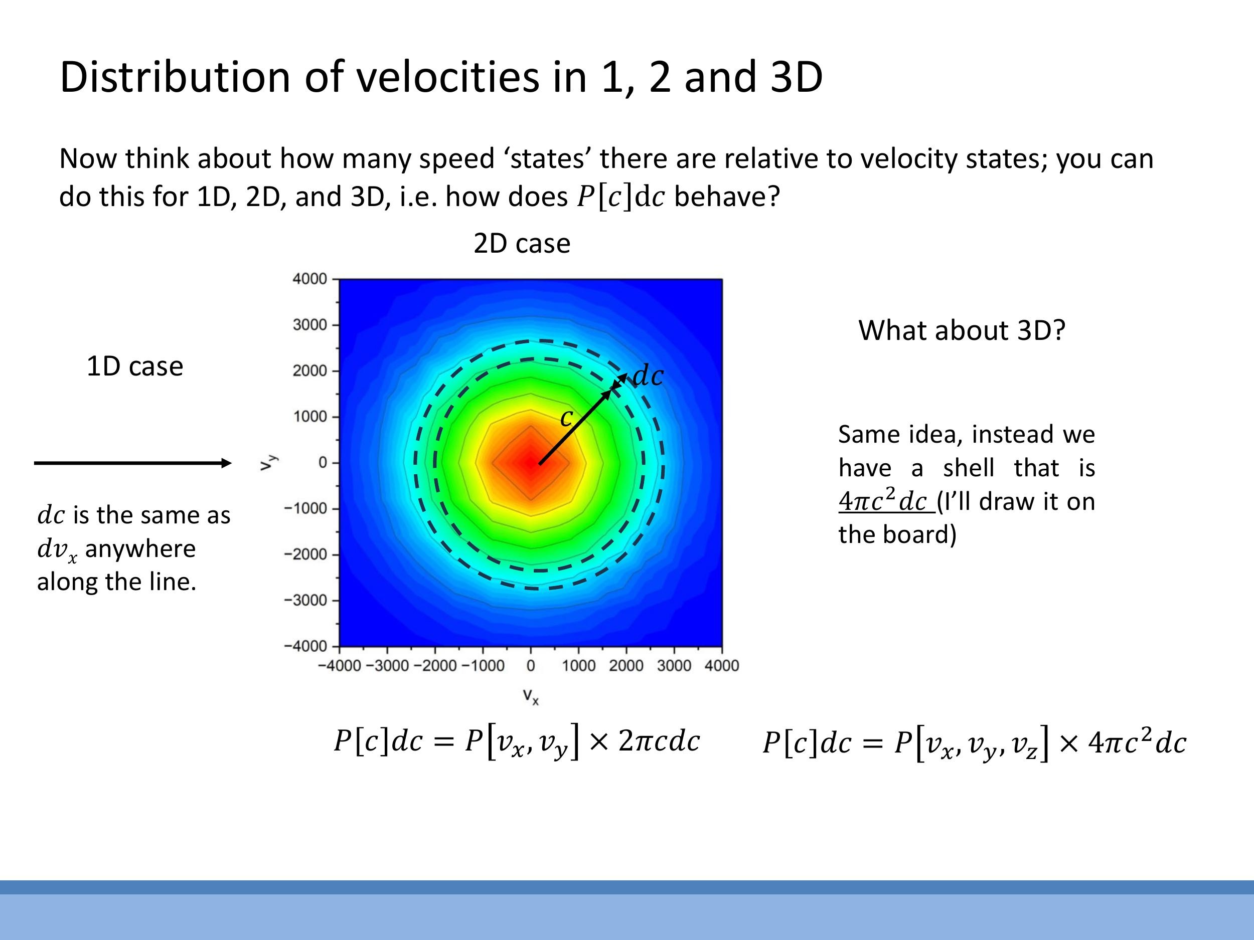
When analysing the motion of gas particles, it is often more physically relevant to consider their speed, $c = \sqrt{v_x^2 + v_y^2 + v_z^2}$, rather than their individual velocity components, $v_x$, $v_y$, and $v_z$. A crucial conceptual step in moving from velocity components to overall speed is understanding how the number of distinct velocity states that share the same speed changes with that speed. This "state counting" or "density of states" depends fundamentally on the geometry of the velocity space.
In one dimension, a small increment in speed $\text{d}c$ directly corresponds to an increment $\text{d}v_x$ along the velocity axis. There is no additional growth factor for the number of states. However, in two dimensions, all velocity states corresponding to a given speed $c$ lie on a circle of radius $c$ in the $v_x$ - $v_y$ plane. The number of such states in a small speed interval $\text{d}c$ is proportional to the circumference of this circle, $2\pi c \, \text{d}c $. Extending this to three dimensions, the velocity states for a given speed $ c $ lie on the surface of a sphere of radius $ c $ in $ v_x $-$ v_y $-$ v_z $ space. Consequently, the number of states in a speed interval $ \text{d}c $ is proportional to the surface area of this sphere, $ 4\pi c^2 \, \text{d}c $. This geometric growth factor means that as speed $ c$ increases, there are quadratically more ways for a particle to achieve that speed. This increasing density of states competes with the exponentially decaying Boltzmann factor, which favours lower energies.
2) Maxwell-Boltzmann speed distribution in 3D: form and shape
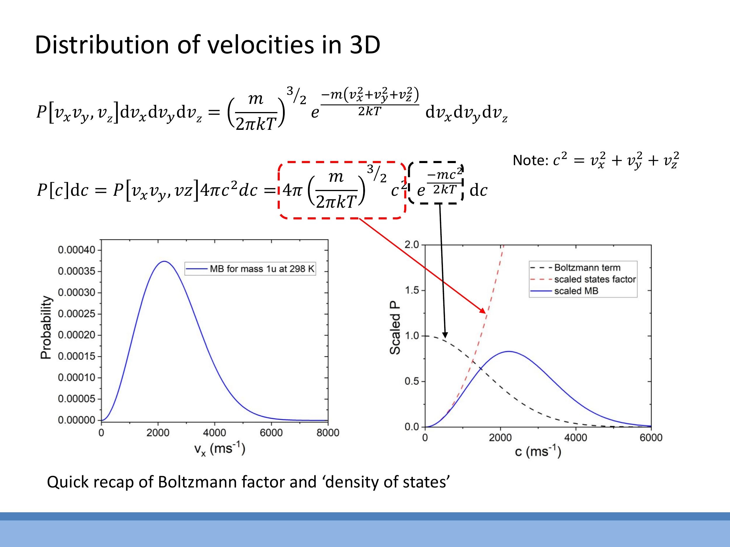
The three-dimensional Maxwell-Boltzmann speed distribution arises from the product of two competing factors. The first is the Boltzmann factor, $e^{-mc^2/2kT}$, which describes the exponential decay in the probability of finding particles at higher energies (and thus higher speeds). This term strongly favours lower speeds. The second factor is the state-counting term, $4\pi c^2$, which represents the increasing number of available velocity states as the speed $c$ increases, as derived from the spherical geometry in velocity space.
Combining these ingredients, the normalised Maxwell-Boltzmann speed distribution $P(c) \, \text{d}c $ for a gas particle of mass $ m $ at temperature $ T$ is given by:
$$
P(c)\,\text{d}c = 4\pi \left( \frac{m}{2\pi kT} \right)^{3/2} c^2 e^{-\frac{mc^2}{2kT}}\,\text{d}c
$$
Here, $k$ is the Boltzmann constant and $c$ is the particle's speed. The shape of this distribution reflects the interplay between these two factors. It starts at $P(c)=0$ for $c=0$ because the $c^2$ term is zero. It then rises as the $c^2$ factor dominates, leading to a peak at the most probable speed. Beyond this peak, the exponential Boltzmann factor, which decays rapidly with $c^2$, eventually dominates, causing the distribution to fall off towards zero at high speeds. This distribution can be used to answer various questions about gas particle speeds, such as determining the most probable speed by finding the maximum of $P(c)$ (i.e., by setting $\frac{\text{d}P}{\text{d}c} = 0$).
3) Average kinetic energy from the 3D distribution: recovering 3/2 kT
To connect the Maxwell-Boltzmann speed distribution to the macroscopic concept of temperature, the average translational kinetic energy per particle is calculated. This is achieved by first determining the mean-square speed, $\overline{c^2}$, from the distribution $P(c) \, \text{d}c$:
$$
\overline{c^2} = \int_0^\infty c^2 P(c)\,\text{d}c
$$
This integral requires the use of standard Gaussian integrals, specifically of the form $\int_0^\infty x^4 e^{-\alpha x^2} \, \text{d}x$, which would typically be provided in reference sheets during examinations. Upon performing this integration, the core result for the mean-square speed is found to be:
$$
\overline{c^2} = \frac{3kT}{m}
$$
Substituting this into the definition of average translational kinetic energy per particle, $\frac{1}{2}m\overline{c^2}$, yields the fundamental result:
$$
\frac{1}{2}m\overline{c^2} = \frac{1}{2}m \left( \frac{3kT}{m} \right) = \frac{3}{2}kT
$$
This result is highly significant as it demonstrates that statistical reasoning, based on the Maxwell-Boltzmann distribution, precisely reproduces the classical thermodynamic result: temperature is a direct measure of the average translational kinetic energy of particles in a system. The focus here is on the physical meaning of this result, with the understanding that complex integrals are provided as tools rather than being primary learning objectives for derivation.
4) Equipartition and internal energy U
The equipartition theorem states that, for a system in thermal equilibrium, each independent quadratic degree of freedom contributes an average energy of $\frac{1}{2}kT$ to the system's total energy. A degree of freedom essentially represents a way in which a molecule can store energy, such as translational motion, rotation, or vibration.
For a monatomic gas, such as helium (He) or argon (Ar), only three translational degrees of freedom (motion along the $x$, $y$, and $z$ axes) are typically active. Therefore, the internal energy per particle is $3 \times \frac{1}{2}kT = \frac{3}{2}kT$. For one mole of a monatomic gas, this translates to an internal energy $U = \frac{3}{2}RT$, where $R$ is the ideal gas constant.
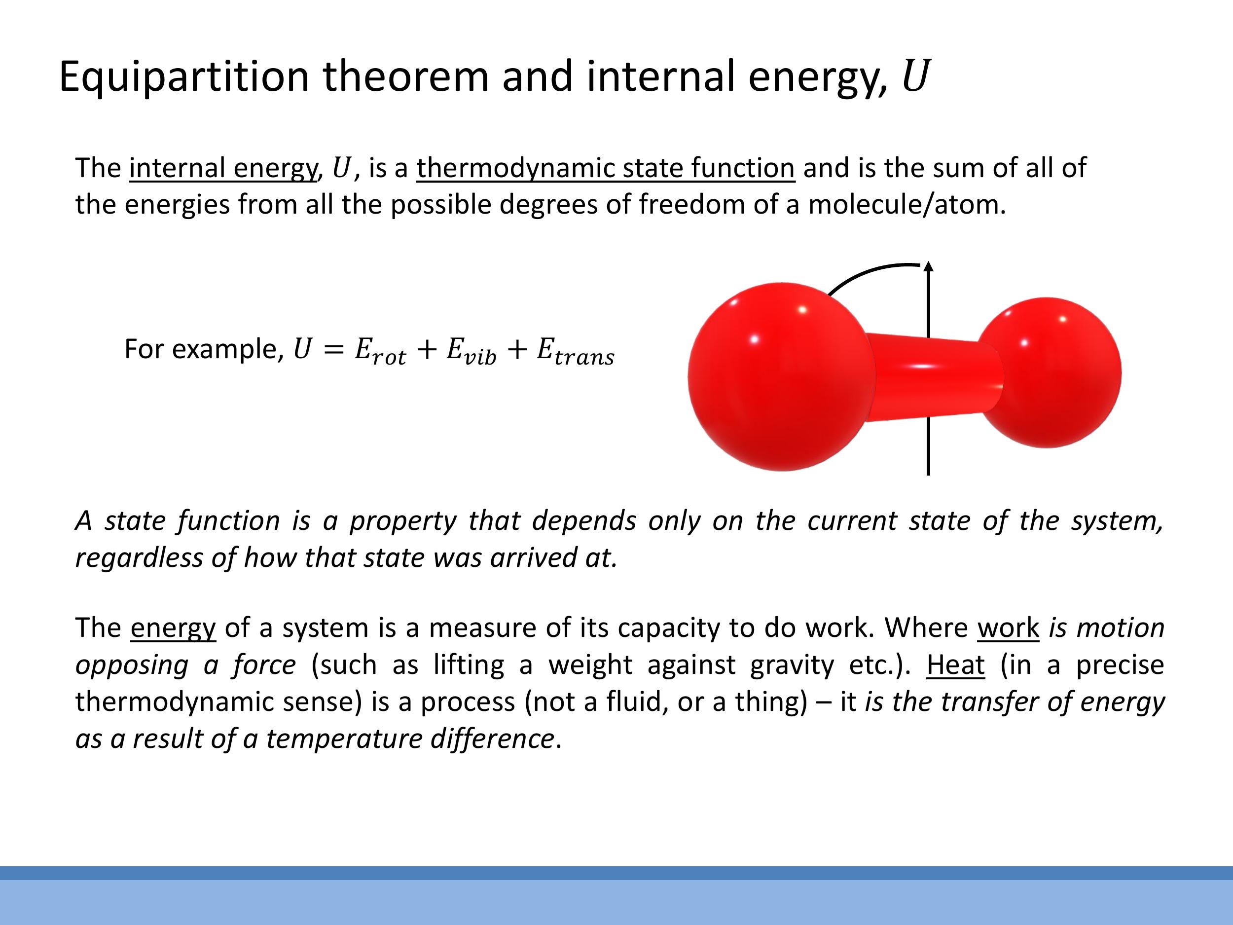
Diatomic gases, like nitrogen ($\text{N}_2$) or oxygen ($\text{O}_2$), possess additional degrees of freedom. At room temperature, they typically exhibit three translational and two rotational degrees of freedom (rotations about two axes perpendicular to the molecular bond), leading to an internal energy of $\frac{5}{2}kT$ per particle. Vibrational modes, which contribute two further degrees of freedom (one for kinetic energy and one for potential energy of the bond), generally require higher temperatures to become active due to larger energy spacing.
The internal energy $U$ of a system is the sum of all accessible energy modes of its constituent particles, including translational, rotational, and vibrational energies ($U = E_{\text{trans}} + E_{\text{rot}} + E_{\text{vib}} + \dots$). Critically, $U$ is a thermodynamic state function, meaning its value depends solely on the current macroscopic state of the system (e.g., its temperature and volume) and not on the particular path taken to reach that state.
5) Microscopic picture: what “work” and “heat” mean
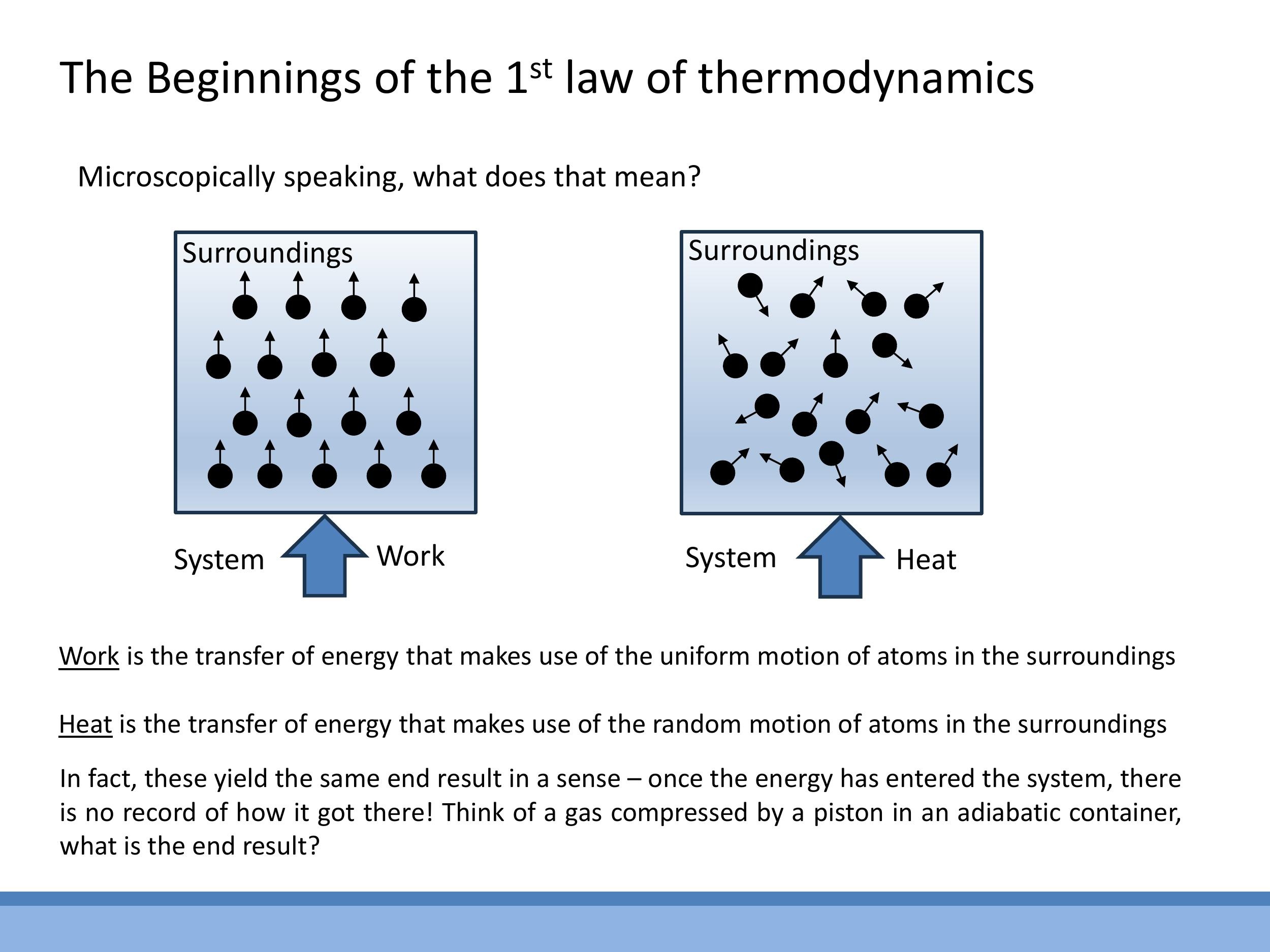
Energy can be transferred into a thermodynamic system through two primary mechanisms: work and heat. At a microscopic level, these two forms of energy transfer are distinguished by the nature of the motion involved. Work involves the transfer of energy through the ordered, uniform motion of particles from the surroundings. A classic example is a piston compressing a gas, where the collective, directed movement of the piston's atoms imparts energy to the gas molecules.
Conversely, heat is the transfer of energy through the random, chaotic thermal motion of particles from the surroundings. For instance, placing a gas container on a hot plate causes the vigorously vibrating atoms of the plate to randomly collide with and transfer energy to the gas molecules. Despite these distinct microscopic pathways of energy transfer, a key principle of thermodynamics is that once energy has entered a system and the system has equilibrated, its internal energy $U$ becomes "memoryless." This means that the final internal energy of the system is the same regardless of whether the energy was initially transferred as work or as heat; $U$ depends only on the system's current state, not on the history of how that state was achieved.
6) The First Law of Thermodynamics: conservation in practice
The First Law of Thermodynamics is a fundamental statement of the conservation of energy, asserting that energy can neither be created nor destroyed, only transformed or transferred. In this course, the First Law is typically expressed in its differential form as:
$$
\text{d}Q = \text{d}U + P\text{d}V
$$
In this equation:
- $\text{d}Q$ represents the infinitesimal amount of heat added to the system.
- $\text{d}U$ represents the infinitesimal change in the system's internal energy.
- $P\text{d}V$ represents the infinitesimal amount of work done by the system on its surroundings due to expansion (where $P$ is pressure and $\text{d}V$ is the change in volume).
Physically, this equation reads: any heat added to a system ($\text{d}Q$) can either increase the system's internal energy ($\text{d}U$) or be used by the system to perform expansion work on its environment ($P\text{d}V$). This formulation reinforces the microscopic understanding from Section 5: heat and work are two distinct processes for transferring energy, both contributing to changes in the system's internal energy. The internal energy $U$ itself is the total microscopic energy (kinetic and potential) of the molecules within the system. For an isolated system, where no heat or work is exchanged with the surroundings, the internal energy $U$ remains constant. It is important to note that various sign conventions for work exist in different texts; this course consistently uses $P\text{d}V$ as work done by the system.
7) Specific heats for an ideal gas: C_V, C_P, and γ
7.1 Constant volume: C_V
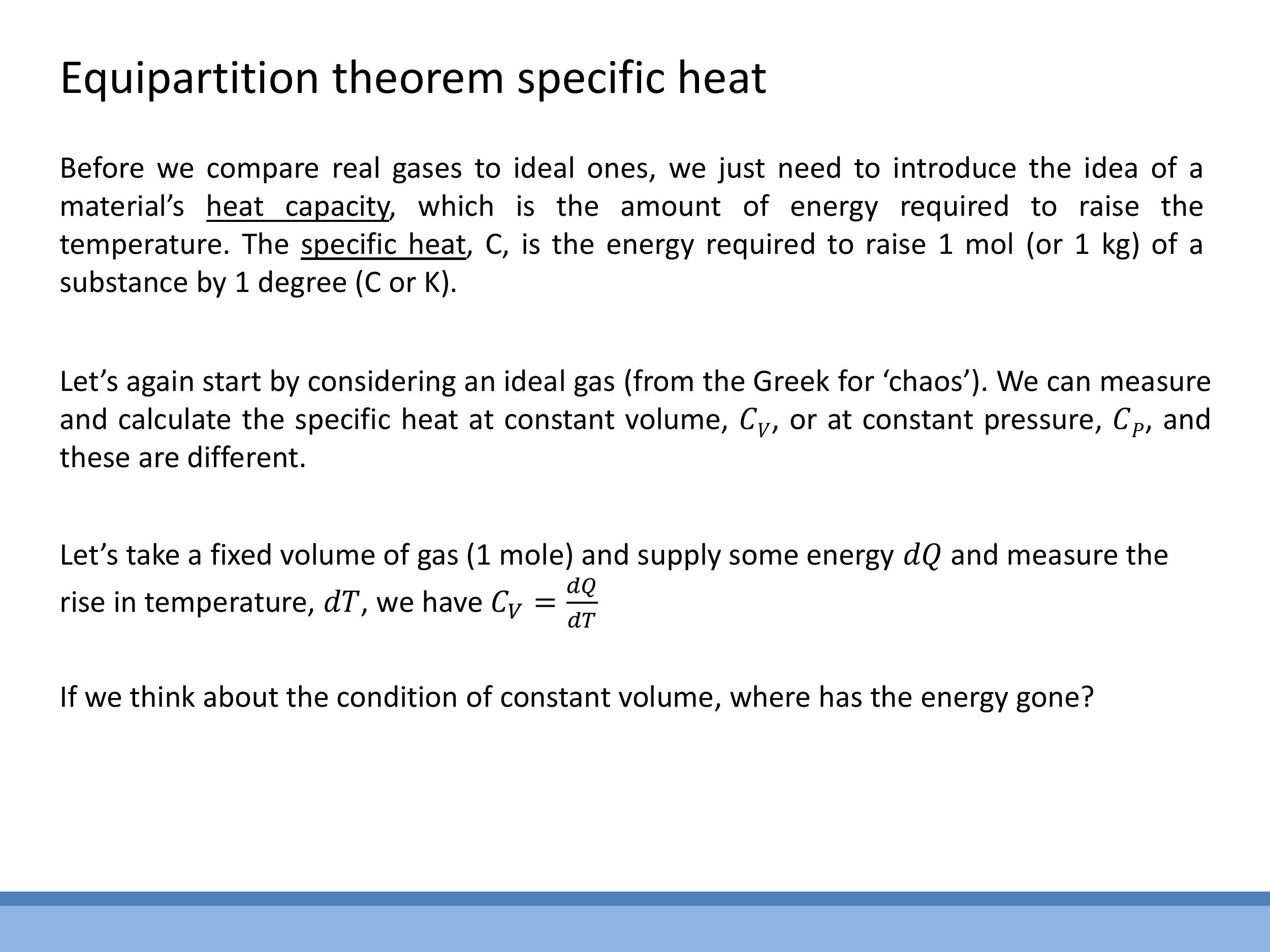
The specific heat capacity at constant volume, $C_V$, quantifies the heat required to raise the temperature of a substance by one degree Kelvin (or Celsius) while its volume is held constant. According to the First Law of Thermodynamics, $\text{d}Q = \text{d}U + P\text{d}V$. If the volume is constant, then $\text{d}V = 0$, which simplifies the First Law to $\text{d}Q = \text{d}U$.
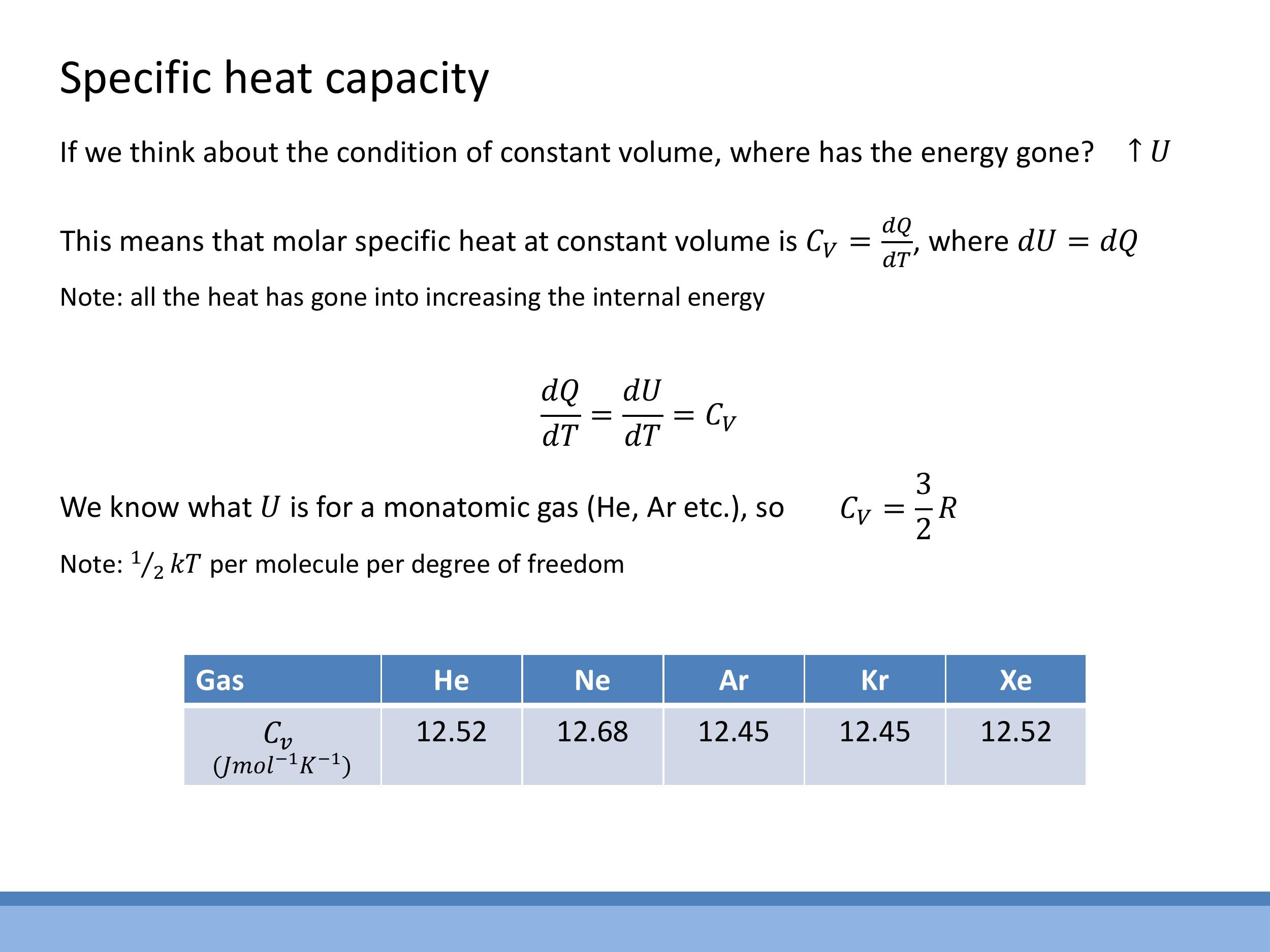
By definition, $C_V = \left(\frac{\text{d}Q}{\text{d}T}\right)_V$. Therefore, for a constant volume process, $C_V = \left(\frac{\text{d}U}{\text{d}T}\right)_V$. For one mole of a monatomic ideal gas, the internal energy is $U = \frac{3}{2}RT$. Differentiating this with respect to temperature $T$ gives the theoretical value for the molar specific heat at constant volume:
$$
C_V = \frac{\text{d}}{\text{d}T}\left(\frac{3}{2}RT\right) = \frac{3}{2}R
$$
Experimental data for noble gases (helium, neon, argon, krypton, xenon) show molar specific heats at constant volume very close to $12.5 \, \text{J mol}^{-1} \, \text{K}^{-1} $, which is in excellent agreement with the theoretical value of $ \frac{3}{2}R $ (where $ R \approx 8.314 \, \text{J mol}^{-1} \, \text{K}^{-1}$). This close agreement is attributed to the weak intermolecular forces in noble gases, which cause them to behave very nearly as ideal gases.
7.2 Constant pressure: C_P and Mayer’s relation
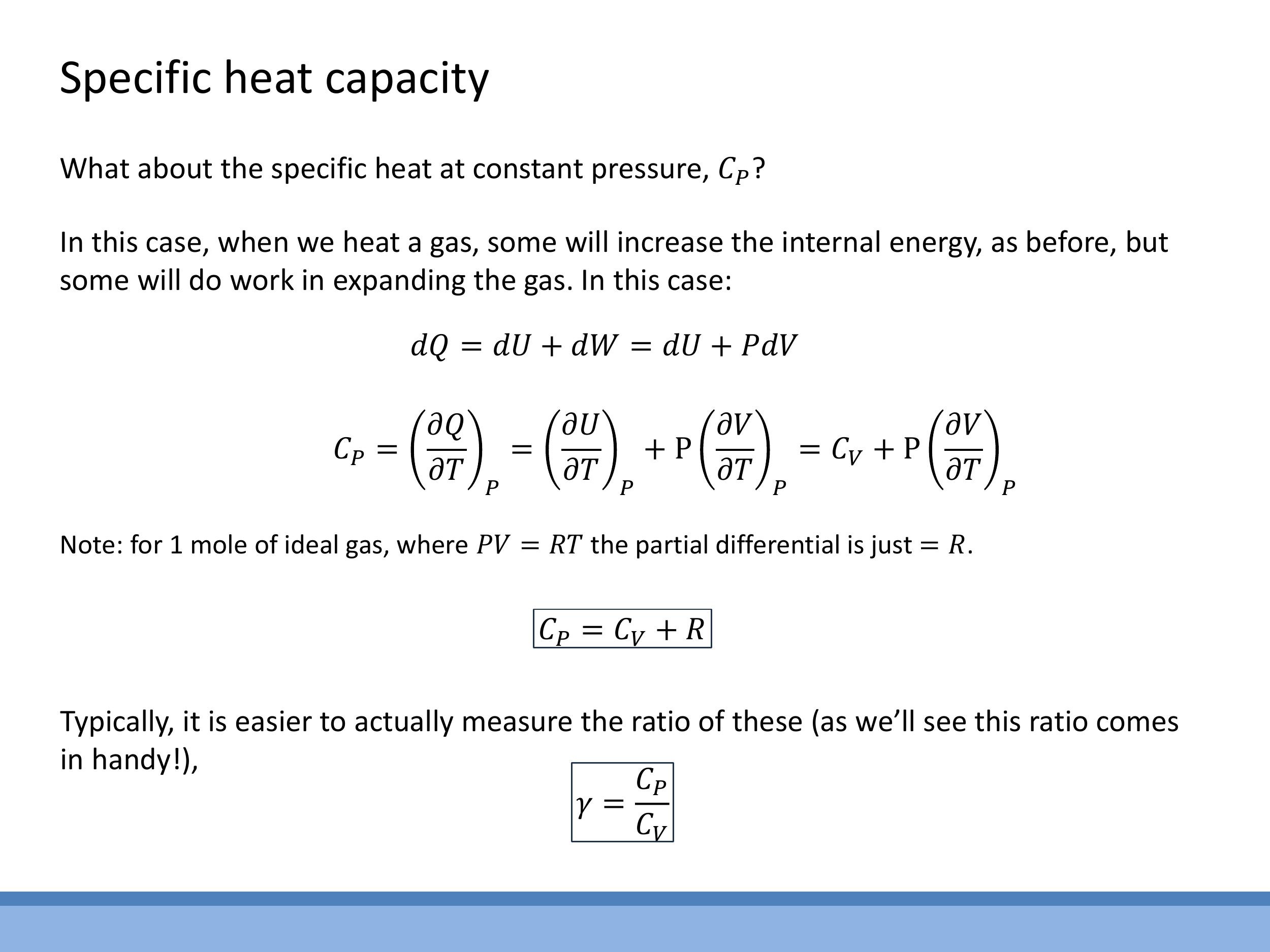
The specific heat capacity at constant pressure, $C_P$, accounts for the heat required to raise the temperature by one degree while maintaining constant pressure. In this process, the gas is typically allowed to expand, meaning work is done by the system. Thus, the full First Law, $\text{d}Q = \text{d}U + P\text{d}V$, must be considered.
$C_P$ is defined as $C_P = \left(\frac{\partial Q}{\partial T}\right)_P$. Applying this to the First Law, we get:
$$
C_P = \left(\frac{\partial U}{\partial T}\right)_P + P\left(\frac{\partial V}{\partial T}\right)_P
$$
The first term, $\left(\frac{\partial U}{\partial T}\right)_P$, is equivalent to $C_V$ (since for an ideal gas, $U$ depends only on $T$, so $\left(\frac{\partial U}{\partial T}\right)_P = \left(\frac{\partial U}{\partial T}\right)_V = C_V$). For the second term, we use the ideal gas law for one mole, $PV = RT$, which can be rearranged to $V = \frac{RT}{P}$. Differentiating $V$ with respect to $T$ at constant $P$ yields $\left(\frac{\partial V}{\partial T}\right)_P = \frac{R}{P}$. Substituting this back into the expression for $C_P$:
$$
C_P = C_V + P\left(\frac{R}{P}\right) = C_V + R
$$
This fundamental relationship, $C_P = C_V + R$, is known as Mayer's relation.
The ratio of specific heats, $\gamma = \frac{C_P}{C_V}$, is a dimensionless quantity that is important in various thermodynamic contexts, such as the speed of sound in a gas. We can calculate $\gamma$ for different ideal gases:
- Monatomic ideal gas: With $C_V = \frac{3}{2}R$ (from 3 translational degrees of freedom) and $C_P = C_V + R = \frac{5}{2}R$, the ratio is $\gamma = \frac{5/2 R}{3/2 R} = \frac{5}{3} \approx 1.67$.
- Diatomic ideal gas at room temperature: With 3 translational and 2 rotational degrees of freedom, $C_V = \frac{5}{2}R$. Using Mayer's relation, $C_P = C_V + R = \frac{7}{2}R$. Thus, $\gamma = \frac{7/2 R}{5/2 R} = \frac{7}{5} = 1.4$.
At higher temperatures, additional vibrational modes in diatomic molecules become active. These additional degrees of freedom increase both $C_V$ and $C_P$, consequently lowering the value of $\gamma$.
Slides present but not covered this lecture (for clarity)
Slides PoM_lecture_7_page_11.jpg, PoM_lecture_7_page_12.jpg, PoM_lecture_7_page_13.jpg, and PoM_lecture_7_page_14.jpg, which cover real gases, the van der Waals equation, and its correction terms, were not discussed in this lecture. This content will be addressed in the subsequent lecture on real gases.
Key takeaways
The three-dimensional Maxwell-Boltzmann speed distribution is a product of two competing factors: a quadratically increasing state-counting factor ($4\pi c^2$) and an exponentially decaying Boltzmann factor ($e^{-mc^2/2kT}$). This combination results in a distribution that starts at zero, rises to a peak, and then decays at higher speeds.
Averaging the kinetic energy using this 3D distribution yields $\overline{c^2} = \frac{3kT}{m}$, which translates to an average translational kinetic energy per particle of $\frac{3}{2}kT$. This result is significant because it statistically reproduces the classical thermodynamic relationship between temperature and average kinetic energy.
The equipartition theorem states that each quadratic degree of freedom contributes an average energy of $\frac{1}{2}kT$ to a system in thermal equilibrium. Monatomic gases primarily possess 3 translational degrees of freedom, while diatomic gases at room temperature typically access 3 translational and 2 rotational degrees of freedom. Vibrational modes become active at higher temperatures. The internal energy $U$ of a system is a state function, representing the sum of energies from all accessible modes.
The First Law of Thermodynamics, in the form $\text{d}Q = \text{d}U + P\text{d}V$, states that heat added to a system can increase its internal energy or be used to perform expansion work. Microscopically, work involves ordered energy transfer, while heat involves random energy transfer. Crucially, once energy is within a system, its contribution to internal energy is indistinguishable regardless of its origin.
For ideal gases, the specific heats are derived as:
- $C_V = \left(\frac{\text{d}U}{\text{d}T}\right)_V$. For monatomic ideal gases, $C_V = \frac{3}{2}R$, a value consistent with experimental data for noble gases.
- $C_P = C_V + R$, known as Mayer's relation.
The ratio of specific heats, $\gamma = \frac{C_P}{C_V}$, is $\frac{5}{3} \approx 1.67$ for monatomic gases and $\frac{7}{5} = 1.4$ for diatomic gases at room temperature. Additional active modes at higher temperatures will alter these specific heat values and their ratio.
## Lecture 7: First Law of Thermodynamics - from Maxwell-Boltzmann to Heat, Work, and Specific Heats

### 0) Orientation and quick review
This lecture bridges the Maxwell-Boltzmann (MB) statistical description of gas particles to the macroscopic principles of thermodynamics, culminating in the First Law and the concept of specific heats. The journey begins by extending the velocity component analysis to the full three-dimensional speed distribution, which allows for the recovery of the classical result for average kinetic energy. This foundation then supports a formalisation of the equipartition theorem and internal energy ($U$), leading directly to the First Law of Thermodynamics, expressed as $\text{d}Q = \text{d}U + P\text{d}V$. The lecture concludes by applying these principles to determine the specific heats at constant volume ($C_V$) and constant pressure ($C_P$) for ideal gases, as well as their ratio, $\gamma$.
The previous lecture established the Boltzmann distribution, which assigns an exponential weighting of $e^{-E/kT}$ to different energy states, an idea often visualised as "balls on shelves." This led to the one-dimensional and two-dimensional Maxwell-Boltzmann distributions, demonstrating that each quadratic degree of freedom contributes an average energy of $\frac{1}{2}kT$. For a two-dimensional system, the total average energy is $kT$. These concepts are further reinforced through workshop exercises that explore equipartition using simplified models. The approach in this lecture prioritises physical intuition and the interpretation of compact formulae, avoiding extensive integral derivations during the lecture itself.
### 1) From velocity components to speed in 3D: state counting

When analysing the motion of gas particles, it is often more physically relevant to consider their speed, $c = \sqrt{v_x^2 + v_y^2 + v_z^2}$, rather than their individual velocity components, $v_x$, $v_y$, and $v_z$. A crucial conceptual step in moving from velocity components to overall speed is understanding how the number of distinct velocity states that share the same speed changes with that speed. This "state counting" or "density of states" depends fundamentally on the geometry of the velocity space.
In one dimension, a small increment in speed $\text{d}c$ directly corresponds to an increment $\text{d}v_x$ along the velocity axis. There is no additional growth factor for the number of states. However, in two dimensions, all velocity states corresponding to a given speed $c$ lie on a circle of radius $c$ in the $v_x$-$v_y$ plane. The number of such states in a small speed interval $\text{d}c$ is proportional to the circumference of this circle, $2\pi c\,\text{d}c$. Extending this to three dimensions, the velocity states for a given speed $c$ lie on the surface of a sphere of radius $c$ in $v_x$-$v_y$-$v_z$ space. Consequently, the number of states in a speed interval $\text{d}c$ is proportional to the surface area of this sphere, $4\pi c^2\,\text{d}c$. This geometric growth factor means that as speed $c$ increases, there are quadratically more ways for a particle to achieve that speed. This increasing density of states competes with the exponentially decaying Boltzmann factor, which favours lower energies.
### 2) Maxwell-Boltzmann speed distribution in 3D: form and shape

The three-dimensional Maxwell-Boltzmann speed distribution arises from the product of two competing factors. The first is the Boltzmann factor, $e^{-mc^2/2kT}$, which describes the exponential decay in the probability of finding particles at higher energies (and thus higher speeds). This term strongly favours lower speeds. The second factor is the state-counting term, $4\pi c^2$, which represents the increasing number of available velocity states as the speed $c$ increases, as derived from the spherical geometry in velocity space.
Combining these ingredients, the normalised Maxwell-Boltzmann speed distribution $P(c)\,\text{d}c$ for a gas particle of mass $m$ at temperature $T$ is given by:
$$ P(c)\,\text{d}c = 4\pi \left( \frac{m}{2\pi kT} \right)^{3/2} c^2 e^{-\frac{mc^2}{2kT}}\,\text{d}c $$
Here, $k$ is the Boltzmann constant and $c$ is the particle's speed. The shape of this distribution reflects the interplay between these two factors. It starts at $P(c)=0$ for $c=0$ because the $c^2$ term is zero. It then rises as the $c^2$ factor dominates, leading to a peak at the most probable speed. Beyond this peak, the exponential Boltzmann factor, which decays rapidly with $c^2$, eventually dominates, causing the distribution to fall off towards zero at high speeds. This distribution can be used to answer various questions about gas particle speeds, such as determining the most probable speed by finding the maximum of $P(c)$ (i.e., by setting $\frac{\text{d}P}{\text{d}c} = 0$).
### 3) Average kinetic energy from the 3D distribution: recovering 3/2 kT
To connect the Maxwell-Boltzmann speed distribution to the macroscopic concept of temperature, the average translational kinetic energy per particle is calculated. This is achieved by first determining the mean-square speed, $\overline{c^2}$, from the distribution $P(c)\,\text{d}c$:
$$ \overline{c^2} = \int_0^\infty c^2 P(c)\,\text{d}c $$
This integral requires the use of standard Gaussian integrals, specifically of the form $\int_0^\infty x^4 e^{-\alpha x^2}\,\text{d}x$, which would typically be provided in reference sheets during examinations. Upon performing this integration, the core result for the mean-square speed is found to be:
$$ \overline{c^2} = \frac{3kT}{m} $$
Substituting this into the definition of average translational kinetic energy per particle, $\frac{1}{2}m\overline{c^2}$, yields the fundamental result:
$$ \frac{1}{2}m\overline{c^2} = \frac{1}{2}m \left( \frac{3kT}{m} \right) = \frac{3}{2}kT $$
This result is highly significant as it demonstrates that statistical reasoning, based on the Maxwell-Boltzmann distribution, precisely reproduces the classical thermodynamic result: temperature is a direct measure of the average translational kinetic energy of particles in a system. The focus here is on the physical meaning of this result, with the understanding that complex integrals are provided as tools rather than being primary learning objectives for derivation.
### 4) Equipartition and internal energy U

The equipartition theorem states that, for a system in thermal equilibrium, each independent quadratic degree of freedom contributes an average energy of $\frac{1}{2}kT$ to the system's total energy. A degree of freedom essentially represents a way in which a molecule can store energy, such as translational motion, rotation, or vibration.
For a monatomic gas, such as helium (He) or argon (Ar), only three translational degrees of freedom (motion along the $x$, $y$, and $z$ axes) are typically active. Therefore, the internal energy per particle is $3 \times \frac{1}{2}kT = \frac{3}{2}kT$. For one mole of a monatomic gas, this translates to an internal energy $U = \frac{3}{2}RT$, where $R$ is the ideal gas constant.
Diatomic gases, like nitrogen ($\text{N}_2$) or oxygen ($\text{O}_2$), possess additional degrees of freedom. At room temperature, they typically exhibit three translational and two rotational degrees of freedom (rotations about two axes perpendicular to the molecular bond), leading to an internal energy of $\frac{5}{2}kT$ per particle. Vibrational modes, which contribute two further degrees of freedom (one for kinetic energy and one for potential energy of the bond), generally require higher temperatures to become active due to larger energy spacing.
The internal energy $U$ of a system is the sum of all accessible energy modes of its constituent particles, including translational, rotational, and vibrational energies ($U = E_{\text{trans}} + E_{\text{rot}} + E_{\text{vib}} + \dots$). Critically, $U$ is a thermodynamic state function, meaning its value depends solely on the current macroscopic state of the system (e.g., its temperature and volume) and not on the particular path taken to reach that state.
### 5) Microscopic picture: what “work” and “heat” mean

Energy can be transferred into a thermodynamic system through two primary mechanisms: work and heat. At a microscopic level, these two forms of energy transfer are distinguished by the nature of the motion involved. Work involves the transfer of energy through the ordered, uniform motion of particles from the surroundings. A classic example is a piston compressing a gas, where the collective, directed movement of the piston's atoms imparts energy to the gas molecules.
Conversely, heat is the transfer of energy through the random, chaotic thermal motion of particles from the surroundings. For instance, placing a gas container on a hot plate causes the vigorously vibrating atoms of the plate to randomly collide with and transfer energy to the gas molecules. Despite these distinct microscopic pathways of energy transfer, a key principle of thermodynamics is that once energy has entered a system and the system has equilibrated, its internal energy $U$ becomes "memoryless." This means that the final internal energy of the system is the same regardless of whether the energy was initially transferred as work or as heat; $U$ depends only on the system's current state, not on the history of how that state was achieved.
### 6) The First Law of Thermodynamics: conservation in practice

The First Law of Thermodynamics is a fundamental statement of the conservation of energy, asserting that energy can neither be created nor destroyed, only transformed or transferred. In this course, the First Law is typically expressed in its differential form as:
$$ \text{d}Q = \text{d}U + P\text{d}V $$
In this equation:
- $\text{d}Q$ represents the infinitesimal amount of heat added to the system.
- $\text{d}U$ represents the infinitesimal change in the system's internal energy.
- $P\text{d}V$ represents the infinitesimal amount of work done *by* the system on its surroundings due to expansion (where $P$ is pressure and $\text{d}V$ is the change in volume).
Physically, this equation reads: any heat added to a system ($\text{d}Q$) can either increase the system's internal energy ($\text{d}U$) or be used by the system to perform expansion work on its environment ($P\text{d}V$). This formulation reinforces the microscopic understanding from Section 5: heat and work are two distinct processes for transferring energy, both contributing to changes in the system's internal energy. The internal energy $U$ itself is the total microscopic energy (kinetic and potential) of the molecules within the system. For an isolated system, where no heat or work is exchanged with the surroundings, the internal energy $U$ remains constant. It is important to note that various sign conventions for work exist in different texts; this course consistently uses $P\text{d}V$ as work done *by* the system.
### 7) Specific heats for an ideal gas: C_V, C_P, and γ

#### 7.1 Constant volume: C_V

The specific heat capacity at constant volume, $C_V$, quantifies the heat required to raise the temperature of a substance by one degree Kelvin (or Celsius) while its volume is held constant. According to the First Law of Thermodynamics, $\text{d}Q = \text{d}U + P\text{d}V$. If the volume is constant, then $\text{d}V = 0$, which simplifies the First Law to $\text{d}Q = \text{d}U$.
By definition, $C_V = \left(\frac{\text{d}Q}{\text{d}T}\right)_V$. Therefore, for a constant volume process, $C_V = \left(\frac{\text{d}U}{\text{d}T}\right)_V$. For one mole of a monatomic ideal gas, the internal energy is $U = \frac{3}{2}RT$. Differentiating this with respect to temperature $T$ gives the theoretical value for the molar specific heat at constant volume:
$$ C_V = \frac{\text{d}}{\text{d}T}\left(\frac{3}{2}RT\right) = \frac{3}{2}R $$
Experimental data for noble gases (helium, neon, argon, krypton, xenon) show molar specific heats at constant volume very close to $12.5\,\text{J mol}^{-1}\,\text{K}^{-1}$, which is in excellent agreement with the theoretical value of $\frac{3}{2}R$ (where $R \approx 8.314\,\text{J mol}^{-1}\,\text{K}^{-1}$). This close agreement is attributed to the weak intermolecular forces in noble gases, which cause them to behave very nearly as ideal gases.
#### 7.2 Constant pressure: C_P and Mayer’s relation

The specific heat capacity at constant pressure, $C_P$, accounts for the heat required to raise the temperature by one degree while maintaining constant pressure. In this process, the gas is typically allowed to expand, meaning work is done by the system. Thus, the full First Law, $\text{d}Q = \text{d}U + P\text{d}V$, must be considered.
$C_P$ is defined as $C_P = \left(\frac{\partial Q}{\partial T}\right)_P$. Applying this to the First Law, we get:
$$ C_P = \left(\frac{\partial U}{\partial T}\right)_P + P\left(\frac{\partial V}{\partial T}\right)_P $$
The first term, $\left(\frac{\partial U}{\partial T}\right)_P$, is equivalent to $C_V$ (since for an ideal gas, $U$ depends only on $T$, so $\left(\frac{\partial U}{\partial T}\right)_P = \left(\frac{\partial U}{\partial T}\right)_V = C_V$). For the second term, we use the ideal gas law for one mole, $PV = RT$, which can be rearranged to $V = \frac{RT}{P}$. Differentiating $V$ with respect to $T$ at constant $P$ yields $\left(\frac{\partial V}{\partial T}\right)_P = \frac{R}{P}$. Substituting this back into the expression for $C_P$:
$$ C_P = C_V + P\left(\frac{R}{P}\right) = C_V + R $$
This fundamental relationship, $C_P = C_V + R$, is known as Mayer's relation.
The ratio of specific heats, $\gamma = \frac{C_P}{C_V}$, is a dimensionless quantity that is important in various thermodynamic contexts, such as the speed of sound in a gas. We can calculate $\gamma$ for different ideal gases:
- **Monatomic ideal gas:** With $C_V = \frac{3}{2}R$ (from 3 translational degrees of freedom) and $C_P = C_V + R = \frac{5}{2}R$, the ratio is $\gamma = \frac{5/2 R}{3/2 R} = \frac{5}{3} \approx 1.67$.
- **Diatomic ideal gas at room temperature:** With 3 translational and 2 rotational degrees of freedom, $C_V = \frac{5}{2}R$. Using Mayer's relation, $C_P = C_V + R = \frac{7}{2}R$. Thus, $\gamma = \frac{7/2 R}{5/2 R} = \frac{7}{5} = 1.4$.
At higher temperatures, additional vibrational modes in diatomic molecules become active. These additional degrees of freedom increase both $C_V$ and $C_P$, consequently lowering the value of $\gamma$.
### Slides present but not covered this lecture (for clarity)
Slides `PoM_lecture_7_page_11.jpg`, `PoM_lecture_7_page_12.jpg`, `PoM_lecture_7_page_13.jpg`, and `PoM_lecture_7_page_14.jpg`, which cover real gases, the van der Waals equation, and its correction terms, were not discussed in this lecture. This content will be addressed in the subsequent lecture on real gases.
## Key takeaways
The three-dimensional Maxwell-Boltzmann speed distribution is a product of two competing factors: a quadratically increasing state-counting factor ($4\pi c^2$) and an exponentially decaying Boltzmann factor ($e^{-mc^2/2kT}$). This combination results in a distribution that starts at zero, rises to a peak, and then decays at higher speeds.
Averaging the kinetic energy using this 3D distribution yields $\overline{c^2} = \frac{3kT}{m}$, which translates to an average translational kinetic energy per particle of $\frac{3}{2}kT$. This result is significant because it statistically reproduces the classical thermodynamic relationship between temperature and average kinetic energy.
The equipartition theorem states that each quadratic degree of freedom contributes an average energy of $\frac{1}{2}kT$ to a system in thermal equilibrium. Monatomic gases primarily possess 3 translational degrees of freedom, while diatomic gases at room temperature typically access 3 translational and 2 rotational degrees of freedom. Vibrational modes become active at higher temperatures. The internal energy $U$ of a system is a state function, representing the sum of energies from all accessible modes.
The First Law of Thermodynamics, in the form $\text{d}Q = \text{d}U + P\text{d}V$, states that heat added to a system can increase its internal energy or be used to perform expansion work. Microscopically, work involves ordered energy transfer, while heat involves random energy transfer. Crucially, once energy is within a system, its contribution to internal energy is indistinguishable regardless of its origin.
For ideal gases, the specific heats are derived as:
- $C_V = \left(\frac{\text{d}U}{\text{d}T}\right)_V$. For monatomic ideal gases, $C_V = \frac{3}{2}R$, a value consistent with experimental data for noble gases.
- $C_P = C_V + R$, known as Mayer's relation.
The ratio of specific heats, $\gamma = \frac{C_P}{C_V}$, is $\frac{5}{3} \approx 1.67$ for monatomic gases and $\frac{7}{5} = 1.4$ for diatomic gases at room temperature. Additional active modes at higher temperatures will alter these specific heat values and their ratio.