Lecture 7: First Law of Thermodynamics - from Maxwell-Boltzmann to Heat, Work, and Specific Heats
0) Orientation and quick review
This lecture concludes our discussion of the Maxwell-Boltzmann (MB) distribution by extending it to three dimensions. We'll examine how the distribution of molecular speeds in a gas leads to the classical result for average kinetic energy, $\frac{3}{2}kT$. Following this, we formalise the equipartition theorem and the concept of internal energy ($U$), leading into the First Law of Thermodynamics, expressed as $\text{d}Q = \text{d}U + P\text{d}V$. Finally, we'll apply these principles to understand the specific heats at constant volume ($C_V$) and constant pressure ($C_P$) for ideal gases, and their ratio, $\gamma$.
In the previous lecture, we introduced the Boltzmann distribution, which describes how particles populate energy levels with an exponential weighting factor of $e^{-E/kT}$. We applied this to one-dimensional and two-dimensional systems, finding an average energy of $\frac{1}{2}kT$ per degree of freedom, totalling $kT$ for two dimensions. The concepts of equipartition are further reinforced in this week's workshops through simple models. Throughout this lecture, the focus will be on building physical intuition, followed by the compact mathematical formulae, without delving into extensive integral calculations during the lecture itself.
1) From velocity components to speed in 3D: state counting
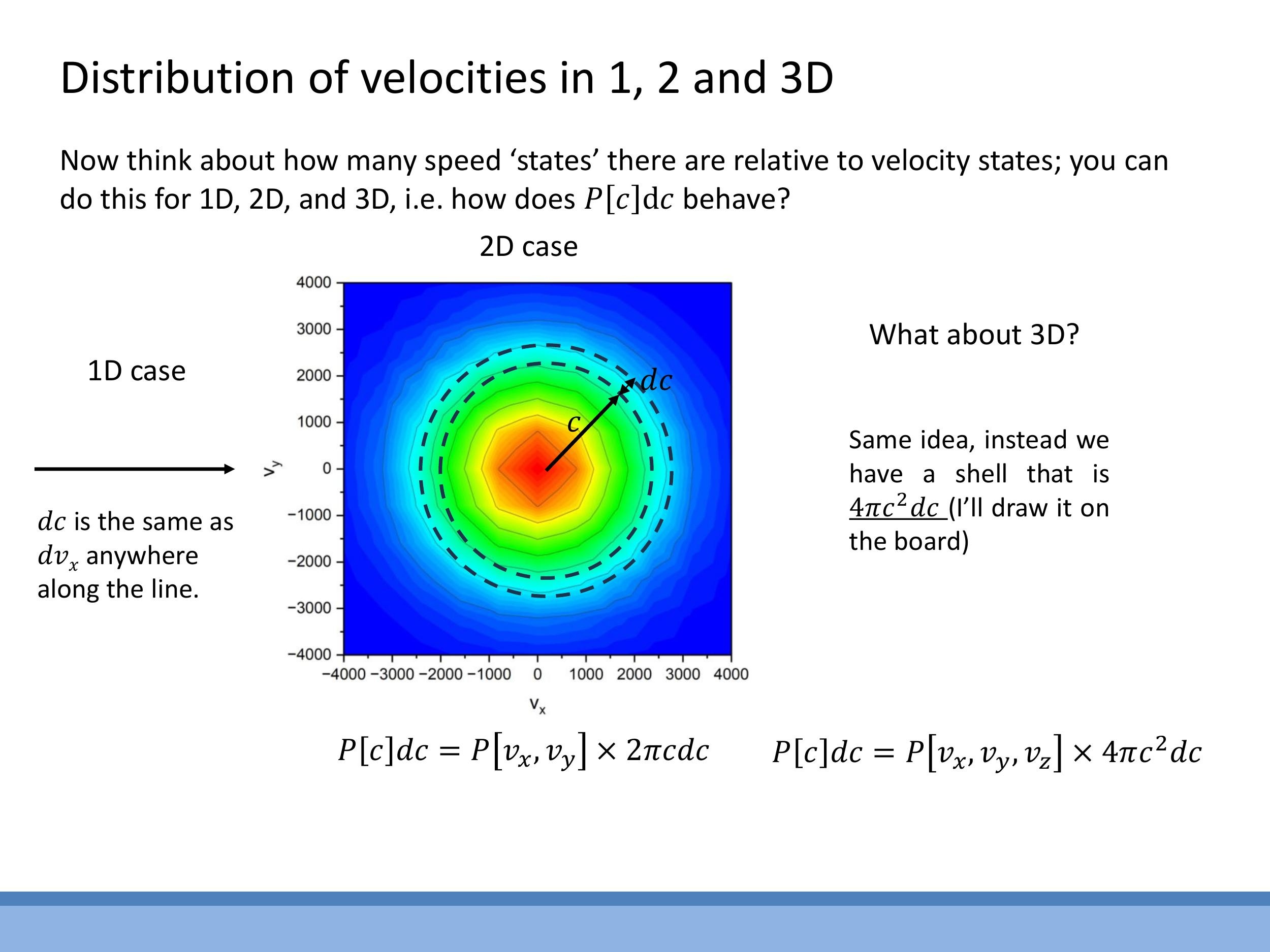
When considering the energy of gas molecules, we are primarily interested in their speeds, $c = \sqrt{v_x^2 + v_y^2 + v_z^2}$, rather than their individual velocity components, which have signed directions. The crucial conceptual step here is that the number of distinct velocity states that correspond to a given speed $c$ increases as $c$ itself increases. This is a geometric effect related to how we count states in velocity space.
To illustrate this, consider the geometry of these "speed states":
- In one dimension, a small interval of speed $\text{d}c$ is directly equivalent to an interval of velocity $\text{d}v_x$. There's no additional growth factor.
- In two dimensions, if we plot $v_x$ against $v_y$, all velocity states corresponding to a given speed $c$ lie on a circle of radius $c$. The number of states within a small speed interval $\text{d}c$ is proportional to the circumference of this circle, which is $2\pi c \, \text{d}c$.
- Extending this to three dimensions, the velocity states for a given speed $c$ lie on the surface of a sphere of radius $c$. The number of states in a small speed interval $\text{d}c$ is proportional to the surface area of this sphere, which is $4\pi c^2 \, \text{d}c$.
This "density of states" factor, $4\pi c^2$, grows quadratically with speed and plays a critical role in shaping the final speed distribution. It effectively competes with the exponentially decaying Boltzmann factor, which favours lower energy states.
2) Maxwell-Boltzmann speed distribution in 3D: form and shape
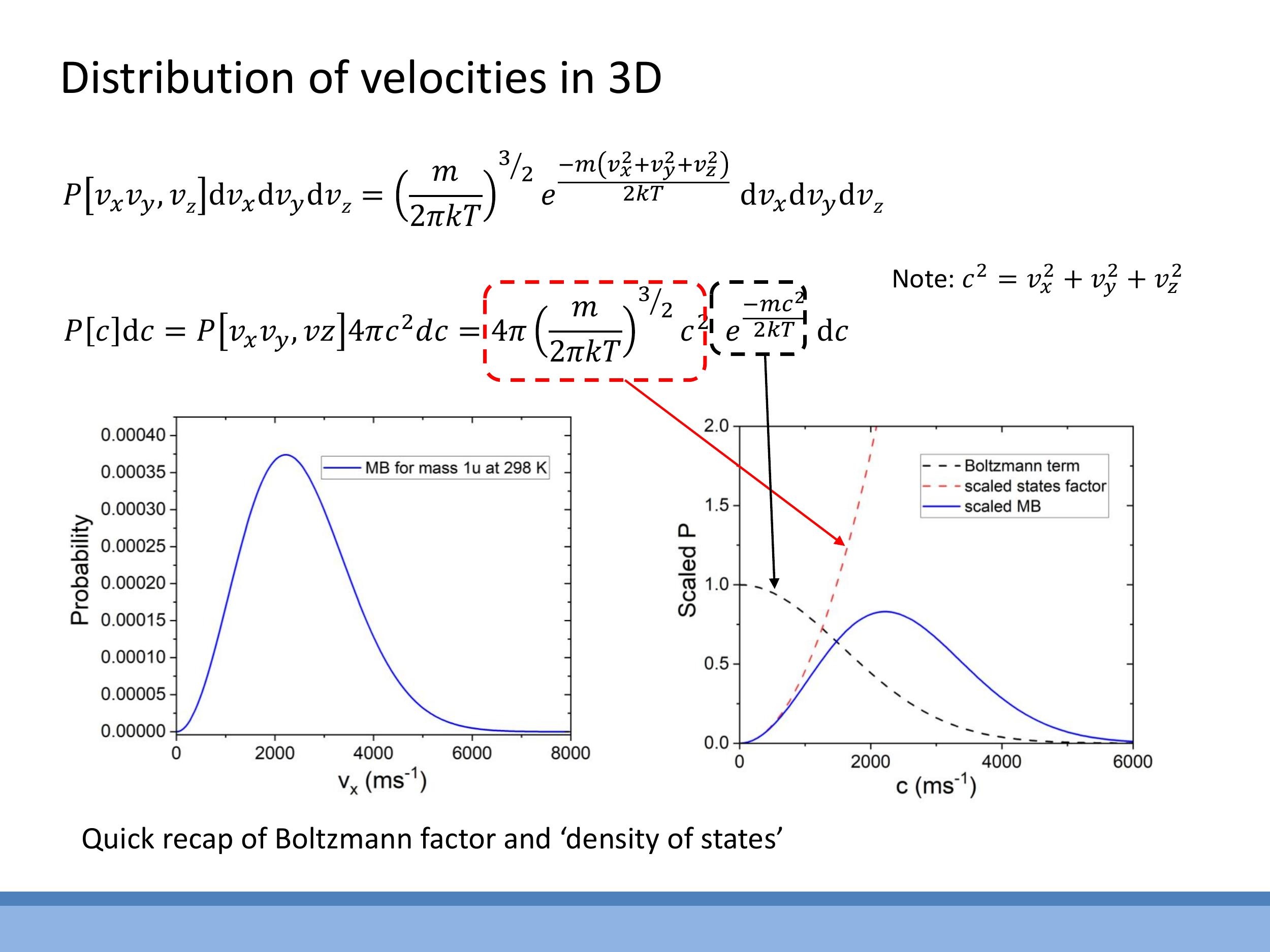
The Maxwell-Boltzmann speed distribution for a gas in three dimensions arises from the combination of two key factors:
- The Boltzmann factor, $e^{-mc^2/2kT}$, which describes the exponential decay in the probability of finding particles at higher energies (and thus higher speeds). This term favours low speeds.
- The state-counting factor, $4\pi c^2$, which we derived from the geometry of velocity space. This term indicates that there are more distinct velocity combinations corresponding to higher speeds, thus favouring higher speeds.
The product of these two competing factors yields the full 3D Maxwell-Boltzmann speed distribution:
$$
P(c)\,\text{d}c = 4\pi \left( \frac{m}{2\pi kT} \right)^{3/2} c^2 e^{-\frac{mc^2}{2kT}}\,\text{d}c
$$
Here, $P(c) \, \text{d}c $ is the probability of a molecule having a speed between $ c $ and $ c+\text{d}c $. $ m $ is the mass of a single molecule, $ k $ is the Boltzmann constant, and $ T$ is the absolute temperature.
The shape of this distribution provides important physical intuition. It starts at $P(c) = 0$ when $c=0$ because the $c^2$ term is zero. As $c$ increases, the $c^2$ factor dominates, causing the probability to rise. It then reaches a peak, representing the most probable speed, after which the exponential Boltzmann factor takes over and causes the distribution to decay rapidly towards zero at very large speeds. This particular shape allows us to answer various questions about gas behaviour, such as determining the most probable speed by finding where $\text{d}P/\text{d}c = 0$.
3) Average kinetic energy from the 3D distribution: recovering 3/2 kT
To solidify the link between the microscopic distribution of speeds and macroscopic temperature, we can use the 3D Maxwell-Boltzmann distribution to calculate the average translational kinetic energy of a gas particle. This involves first computing the mean-square speed, $\overline{c^2}$.
The strategy is to integrate the square of the speed, $c^2$, weighted by the probability distribution $P(c)$, over all possible speeds from zero to infinity:
$$
\overline{c^2} = \int_0^\infty c^2 P(c)\,\text{d}c
$$
This integral requires the use of a standard integral of the form $\int_0^\infty x^4 e^{-\alpha x^2} \, \text{d}x$, which would typically be provided in reference sheets for examinations.
After performing this integration, the core result for the mean-square speed is:
$$
\overline{c^2} = \frac{3kT}{m}
$$
From this, the average translational kinetic energy per particle can be directly calculated:
$$
\frac{1}{2}m\overline{c^2} = \frac{1}{2}m \left( \frac{3kT}{m} \right) = \frac{3}{2}kT
$$
This result is significant because it shows that statistical, Maxwell-Boltzmann reasoning precisely reproduces the classical thermodynamic result for the average translational kinetic energy of an ideal gas particle. In essence, temperature is a direct measure of this average translational kinetic energy.
4) Equipartition and internal energy U
The equipartition theorem provides a simple and powerful statement about how energy is distributed in a system at thermal equilibrium: each quadratic degree of freedom contributes an average energy of $\frac{1}{2}kT$. A quadratic degree of freedom refers to any way a particle can store energy that is proportional to the square of a coordinate or a momentum, such as the kinetic energy associated with motion in one direction ($\frac{1}{2}mv_x^2$).
Let's look at examples of degrees of freedom:
- A monatomic gas, like helium or argon, consists of single atoms. These atoms can only move translationally in three independent directions (x, y, and z). Therefore, a monatomic gas has 3 translational degrees of freedom, leading to a total internal energy per particle of $3 \times \frac{1}{2}kT = \frac{3}{2}kT$. Per mole, this becomes $\frac{3}{2}RT$.
- A diatomic gas, such as nitrogen ($\text{N}_2$) or oxygen ($\text{O}_2$), has additional ways to store energy. At room temperature, it typically has 3 translational degrees of freedom and 2 rotational degrees of freedom (rotation about two axes perpendicular to the molecular bond). Vibrational modes, which involve the atoms oscillating along the bond (contributing both kinetic and potential energy, thus 2 additional degrees of freedom), usually require higher temperatures to become active due to larger energy spacing.
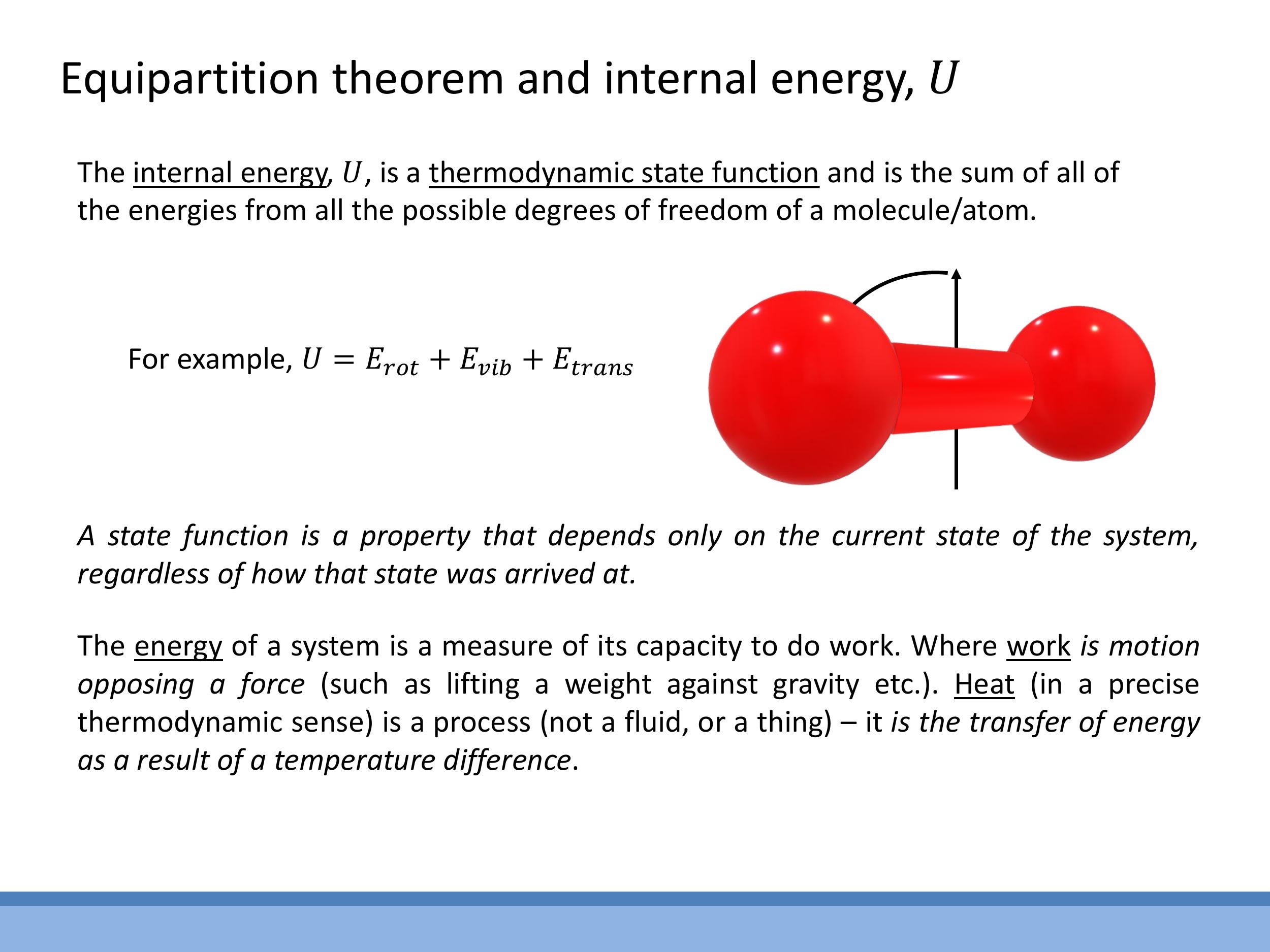
The internal energy ($U$) of a system is the sum of all accessible energy modes of its constituent particles, including translational, rotational, and vibrational energies ($U = E_{\text{trans}} + E_{\text{rot}} + E_{\text{vib}} + \dots$). A key property of internal energy is that it is a thermodynamic state function
5) Microscopic picture: what “work” and “heat” mean
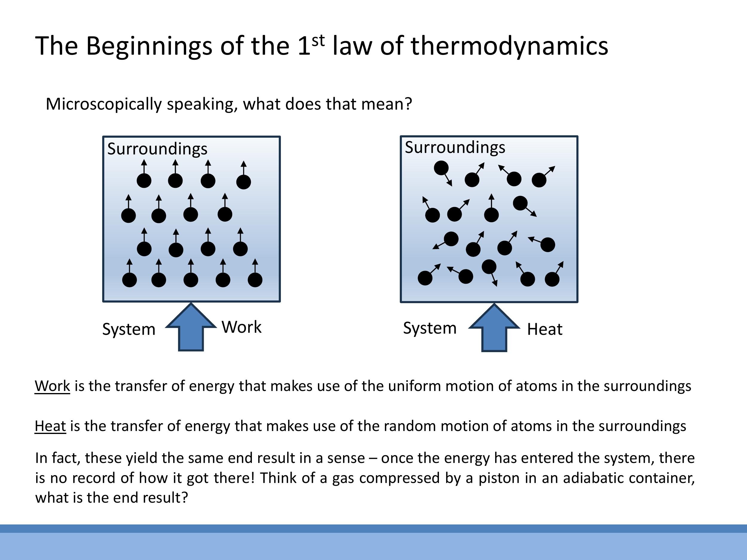
From a microscopic perspective, energy can be transferred into a system in two fundamental ways: as work or as heat.
- Work involves the transfer of energy through the ordered, uniform motion of atoms or molecules in the surroundings. Imagine a piston compressing a gas: the piston's collective, directional motion transfers energy to the gas molecules, increasing their internal energy.
- Heat involves the transfer of energy through the random, chaotic motion of atoms or molecules in the surroundings. Consider a hot plate transferring energy to a gas: the vigorously vibrating atoms of the hot plate randomly collide with the gas molecules, increasing their disordered thermal motion and thus their internal energy.
A crucial insight is that once energy has been transferred into the system, its effect on the internal energy ($U$) is indistinguishable, regardless of whether it entered as work or as heat. The system has no "memory" of the energy's origin. The internal energy $U$ is a state function that solely depends on the system's current state, not on the pathway that led to that state.
6) The First Law of Thermodynamics: conservation in practice
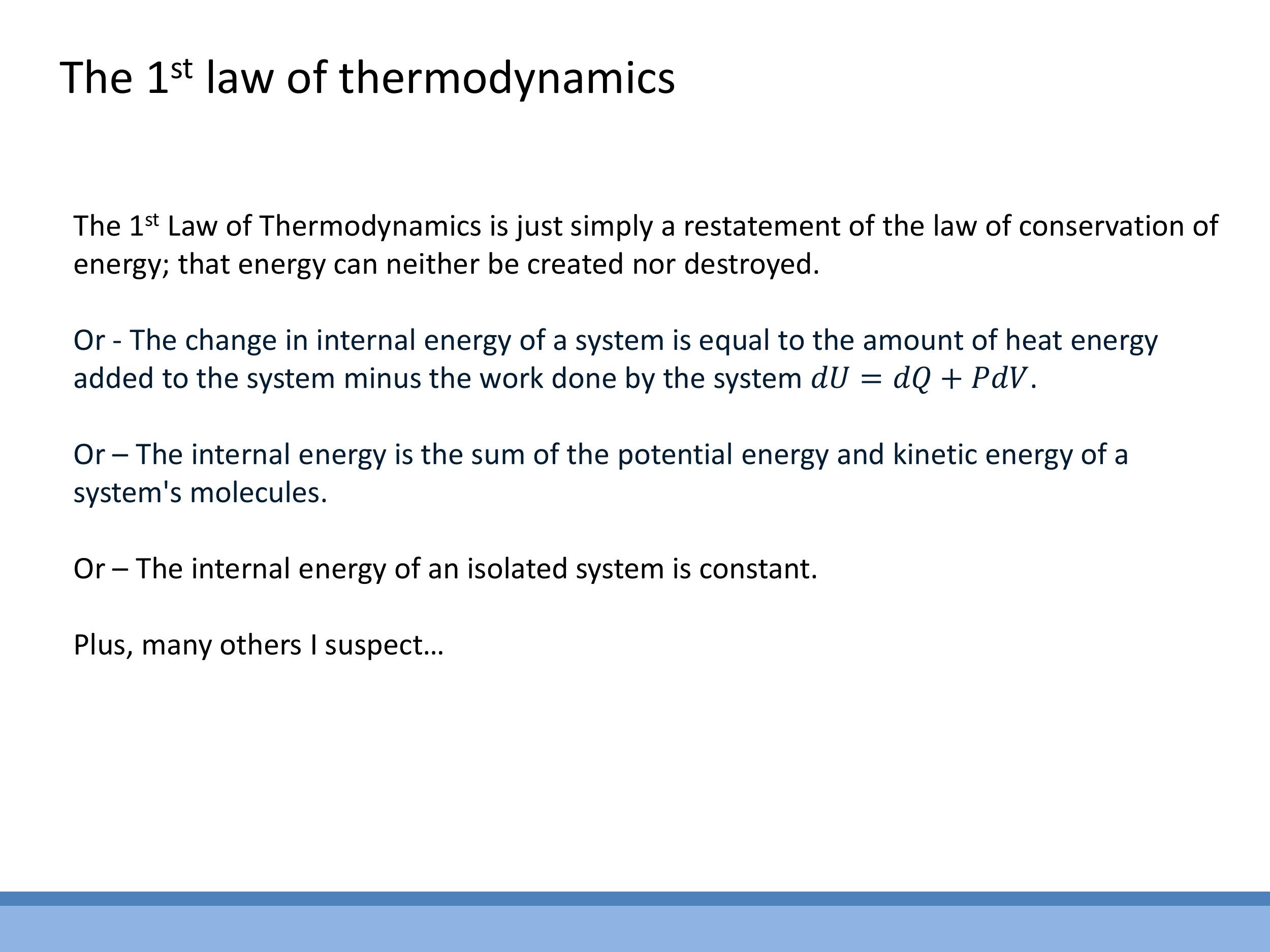
The First Law of Thermodynamics is a statement of the conservation of energy, adapted for thermodynamic systems. It quantifies how energy is transferred and transformed. In this course, we will consistently use the following form:
$$
\text{d}Q = \text{d}U + P\text{d}V
$$
This equation can be read as: the heat added to the system ($\text{d}Q$) can either increase the system's internal energy ($\text{d}U$) or be used by the system to do expansion work on its surroundings ($P\text{d}V$). This form defines $P\text{d}V$ as the work done by the system.
In this context, $U$ represents the total microscopic energy of the molecules within the system, encompassing both their kinetic and potential energies. For an isolated system, where no energy or matter can be exchanged with the surroundings ($\text{d}Q = 0$ and $P\text{d}V = 0$), the First Law implies that the internal energy $U$ remains constant. It's important to adhere to the chosen sign convention for this course to avoid confusion.
7) Specific heats for an ideal gas: C_V, C_P, and γ
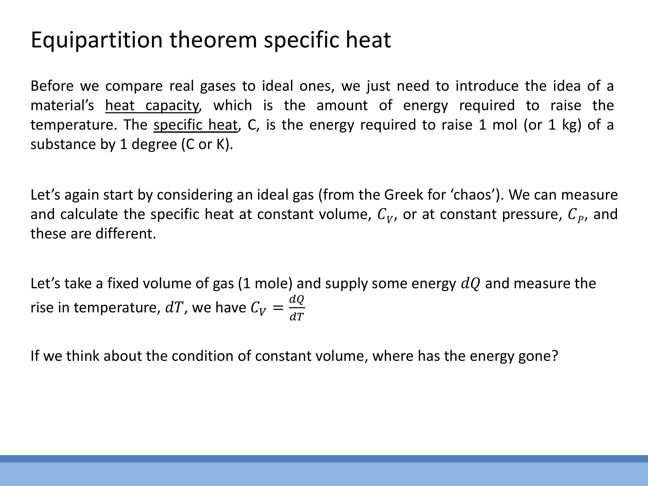
Heat capacity is a macroscopic property that quantifies the amount of energy required to raise the temperature of a material. When considering a specific quantity of matter, such as one mole, we refer to it as molar specific heat ($C$). Two important specific heats are defined: at constant volume ($C_V$) and at constant pressure ($C_P$).
7.1 Constant volume: C_V
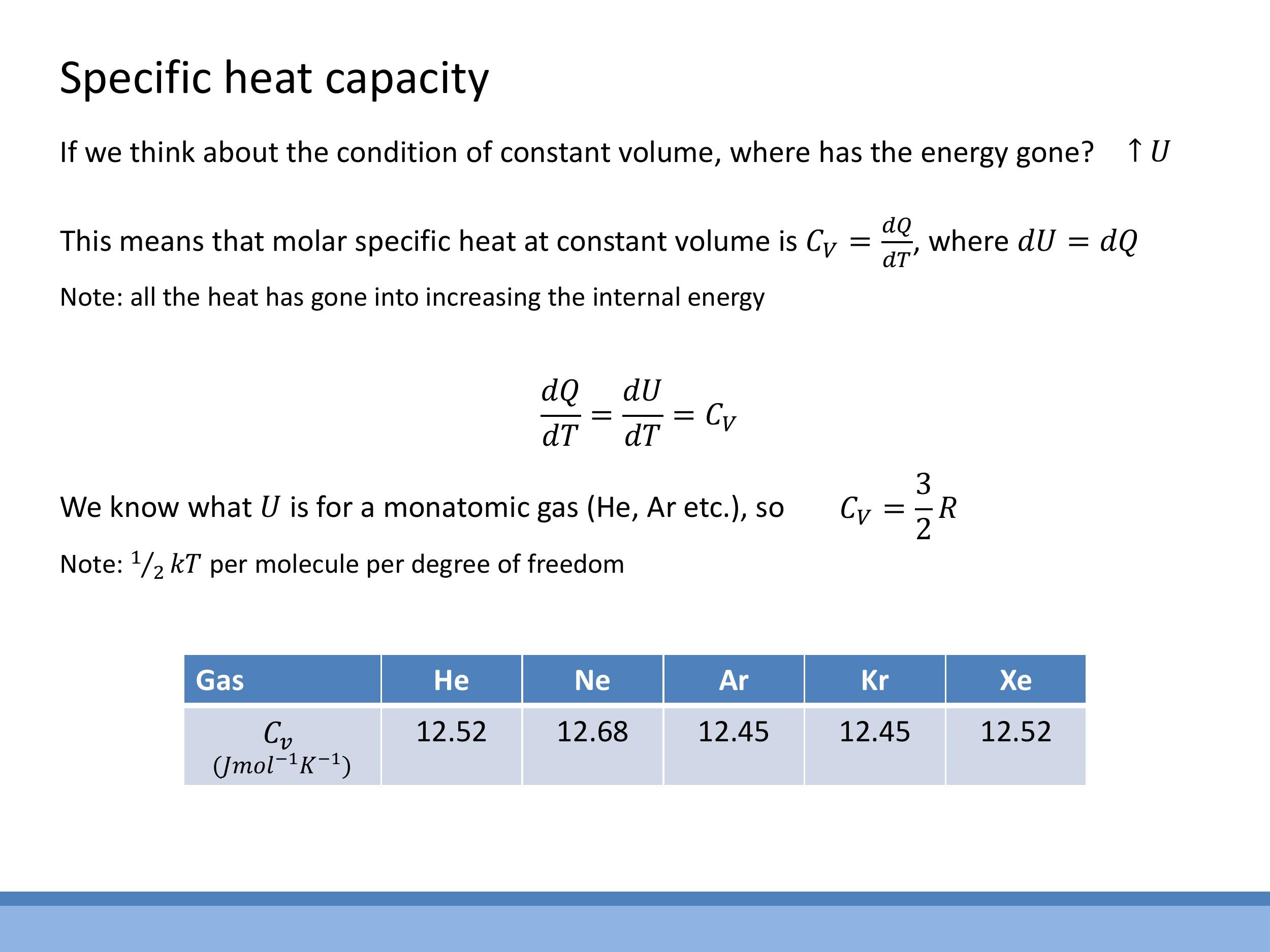
For a process occurring at constant volume, the volume change $\text{d}V$ is zero. This simplifies the First Law of Thermodynamics to $\text{d}Q = \text{d}U$, as no expansion work is done. The molar specific heat at constant volume, $C_V$, is defined as the heat added per unit temperature change at constant volume: $C_V = \left(\frac{\text{d}Q}{\text{d}T}\right)_V$. Consequently, for a constant volume process, $C_V = \left(\frac{\text{d}U}{\text{d}T}\right)_V$.
For one mole of a monatomic ideal gas, the internal energy $U$ is given by $U = \frac{3}{2}RT$, where $R$ is the ideal gas constant. Differentiating this expression with respect to temperature $T$ yields the theoretical value for $C_V$:
$$
C_V = \frac{3}{2}R
$$
This theoretical prediction is remarkably well-supported by experimental data for noble gases (like helium, neon, and argon), which behave very closely to ideal monatomic gases due to their weak intermolecular forces. Their measured $C_V$ values are approximately $12.5 \, \text{J mol}^{-1} \, \text{K}^{-1} $, which is in close agreement with $ \frac{3}{2}R$.
7.2 Constant pressure: C_P and Mayer’s relation
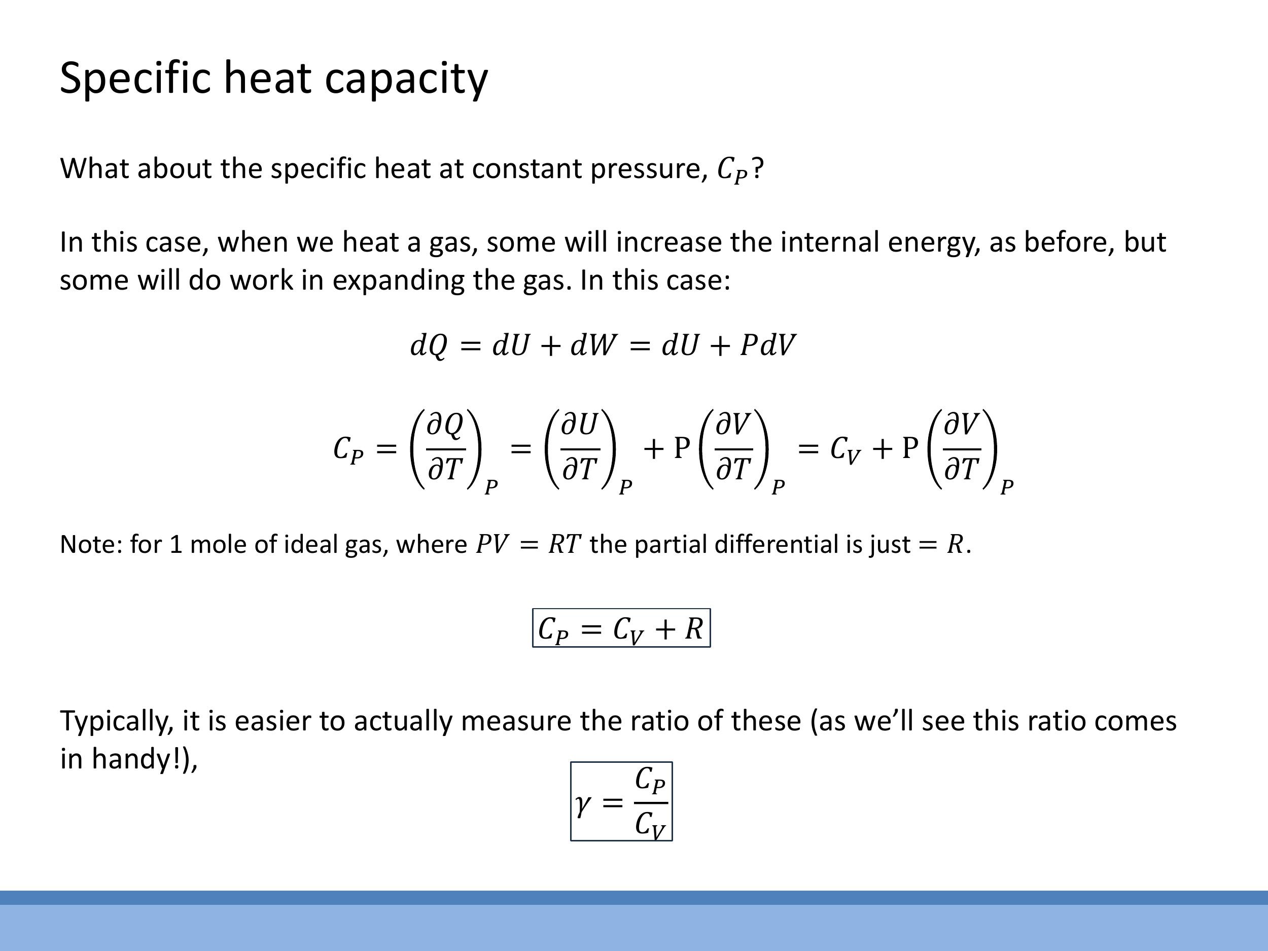
When a gas is heated at constant pressure, it expands and does work on its surroundings. Therefore, the full First Law, $\text{d}Q = \text{d}U + P\text{d}V$, must be considered. The specific heat at constant pressure, $C_P$, is defined as $C_P = \left(\frac{\partial Q}{\partial T}\right)_P$. Applying the First Law, this becomes:
$$
C_P = \left(\frac{\partial U}{\partial T}\right)_P + P\left(\frac{\partial V}{\partial T}\right)_P
$$
The first term, $\left(\frac{\partial U}{\partial T}\right)_P$, is equivalent to $C_V$ for an ideal gas, as the internal energy of an ideal gas depends only on temperature. For the second term, we use the ideal gas law for one mole, $PV = RT$. Rearranging this for volume, $V = \frac{RT}{P}$, and differentiating with respect to temperature $T$ at constant pressure $P$, we get $\left(\frac{\partial V}{\partial T}\right)_P = \frac{R}{P}$. Substituting this back into the expression for $C_P$, the work term $P\left(\frac{\partial V}{\partial T}\right)_P$ simplifies to $P\left(\frac{R}{P}\right) = R$.
This derivation leads to Mayer’s relation:
$$
C_P = C_V + R
$$
Another important quantity is the ratio of specific heats, $\gamma$, which is a dimensionless value defined as:
$$
\gamma = \frac{C_P}{C_V}
$$
We can compute $\gamma$ for different ideal gases:
- For a monatomic ideal gas, $C_V = \frac{3}{2}R$ and $C_P = \frac{3}{2}R + R = \frac{5}{2}R$. Thus, $\gamma = \frac{5/2 R}{3/2 R} = \frac{5}{3} \approx 1.67$.
- For a diatomic gas at room temperature, which typically accesses 3 translational and 2 rotational degrees of freedom (total 5 degrees of freedom), $C_V = \frac{5}{2}R$ and $C_P = \frac{5}{2}R + R = \frac{7}{2}R$. This gives $\gamma = \frac{7/2 R}{5/2 R} = \frac{7}{5} = 1.4$.
It's important to note that if the temperature is high enough to activate additional vibrational modes in diatomic molecules, their $C_V$ and $C_P$ values will increase further, leading to a lower value of $\gamma$.
Slides present but not covered this lecture (for clarity)
Please note that slides PoM_lecture_7_page_11.jpg (Real gases overview), PoM_lecture_7_page_12.jpg (Ideal vs real isotherms), PoM_lecture_7_page_13.jpg (Finite-size correction $b$), and PoM_lecture_7_page_14.jpg (Attractive correction $a$) were not covered in this lecture. Their content, which pertains to real gases, will be addressed in the next lecture.
Key takeaways
The 3D Maxwell-Boltzmann speed distribution is a product of two competing factors: a states factor ($4\pi c^2$) that grows quadratically with speed and an exponential Boltzmann decay factor ($e^{-mc^2/2kT}$) that suppresses high speeds. This combination results in a distribution that rises from zero, peaks at an intermediate speed, and then tails off.
By averaging with this 3D distribution, we find that the mean-square speed $\overline{c^2} = \frac{3kT}{m}$, which means the average translational kinetic energy per particle is $\frac{3}{2}kT$. This result is a fundamental link between microscopic particle motion and macroscopic temperature, matching classical predictions.
The equipartition theorem states that each quadratic degree of freedom in a system at thermal equilibrium contributes an average energy of $\frac{1}{2}kT$. For monatomic gases, this means 3 translational degrees of freedom, while diatomic gases at room temperature also include 2 rotational degrees of freedom. Vibrational modes become active at higher temperatures.
Internal energy ($U$) is a thermodynamic state function that represents the sum of all accessible energy modes within a system. Its value depends only on the system's current state, not on the path taken to reach it.
The First Law of Thermodynamics, in the form used in this course, is $\text{d}Q = \text{d}U + P\text{d}V$. This equation shows that heat added to a system ($\text{d}Q$) can either increase its internal energy ($\text{d}U$) or be used by the system to do expansion work ($P\text{d}V$). Microscopically, heat and work are distinct pathways for energy transfer, but once the energy is within the system, it is indistinguishable in its contribution to internal energy.
For ideal gases, we derive specific heats:
- At constant volume, $C_V = \left(\frac{\text{d}U}{\text{d}T}\right)_V$. For monatomic ideal gases, $C_V = \frac{3}{2}R$, a value consistent with experimental data for noble gases.
- At constant pressure, $C_P = C_V + R$, known as Mayer's relation.
The ratio of specific heats, $\gamma = \frac{C_P}{C_V}$, is $\frac{5}{3}$ for monatomic gases and $1.4$ for diatomic gases at room temperature. The activation of additional energy modes at higher temperatures will alter these values.
## Lecture 7: First Law of Thermodynamics - from Maxwell-Boltzmann to Heat, Work, and Specific Heats

### 0) Orientation and quick review
This lecture concludes our discussion of the Maxwell-Boltzmann (MB) distribution by extending it to three dimensions. We'll examine how the distribution of molecular speeds in a gas leads to the classical result for average kinetic energy, $\frac{3}{2}kT$. Following this, we formalise the equipartition theorem and the concept of internal energy ($U$), leading into the First Law of Thermodynamics, expressed as $\text{d}Q = \text{d}U + P\text{d}V$. Finally, we'll apply these principles to understand the specific heats at constant volume ($C_V$) and constant pressure ($C_P$) for ideal gases, and their ratio, $\gamma$.
In the previous lecture, we introduced the Boltzmann distribution, which describes how particles populate energy levels with an exponential weighting factor of $e^{-E/kT}$. We applied this to one-dimensional and two-dimensional systems, finding an average energy of $\frac{1}{2}kT$ per degree of freedom, totalling $kT$ for two dimensions. The concepts of equipartition are further reinforced in this week's workshops through simple models. Throughout this lecture, the focus will be on building physical intuition, followed by the compact mathematical formulae, without delving into extensive integral calculations during the lecture itself.
### 1) From velocity components to speed in 3D: state counting

When considering the energy of gas molecules, we are primarily interested in their speeds, $c = \sqrt{v_x^2 + v_y^2 + v_z^2}$, rather than their individual velocity components, which have signed directions. The crucial conceptual step here is that the number of distinct velocity states that correspond to a given speed $c$ increases as $c$ itself increases. This is a geometric effect related to how we count states in velocity space.
To illustrate this, consider the geometry of these "speed states":
* In one dimension, a small interval of speed $\text{d}c$ is directly equivalent to an interval of velocity $\text{d}v_x$. There's no additional growth factor.
* In two dimensions, if we plot $v_x$ against $v_y$, all velocity states corresponding to a given speed $c$ lie on a circle of radius $c$. The number of states within a small speed interval $\text{d}c$ is proportional to the circumference of this circle, which is $2\pi c\,\text{d}c$.
* Extending this to three dimensions, the velocity states for a given speed $c$ lie on the surface of a sphere of radius $c$. The number of states in a small speed interval $\text{d}c$ is proportional to the surface area of this sphere, which is $4\pi c^2\,\text{d}c$.
This "density of states" factor, $4\pi c^2$, grows quadratically with speed and plays a critical role in shaping the final speed distribution. It effectively competes with the exponentially decaying Boltzmann factor, which favours lower energy states.
### 2) Maxwell-Boltzmann speed distribution in 3D: form and shape

The Maxwell-Boltzmann speed distribution for a gas in three dimensions arises from the combination of two key factors:
* The **Boltzmann factor**, $e^{-mc^2/2kT}$, which describes the exponential decay in the probability of finding particles at higher energies (and thus higher speeds). This term favours low speeds.
* The **state-counting factor**, $4\pi c^2$, which we derived from the geometry of velocity space. This term indicates that there are more distinct velocity combinations corresponding to higher speeds, thus favouring higher speeds.
The product of these two competing factors yields the full 3D Maxwell-Boltzmann speed distribution:
$$ P(c)\,\text{d}c = 4\pi \left( \frac{m}{2\pi kT} \right)^{3/2} c^2 e^{-\frac{mc^2}{2kT}}\,\text{d}c $$
Here, $P(c)\,\text{d}c$ is the probability of a molecule having a speed between $c$ and $c+\text{d}c$. $m$ is the mass of a single molecule, $k$ is the Boltzmann constant, and $T$ is the absolute temperature.
The shape of this distribution provides important physical intuition. It starts at $P(c) = 0$ when $c=0$ because the $c^2$ term is zero. As $c$ increases, the $c^2$ factor dominates, causing the probability to rise. It then reaches a peak, representing the most probable speed, after which the exponential Boltzmann factor takes over and causes the distribution to decay rapidly towards zero at very large speeds. This particular shape allows us to answer various questions about gas behaviour, such as determining the most probable speed by finding where $\text{d}P/\text{d}c = 0$.
### 3) Average kinetic energy from the 3D distribution: recovering 3/2 kT
To solidify the link between the microscopic distribution of speeds and macroscopic temperature, we can use the 3D Maxwell-Boltzmann distribution to calculate the average translational kinetic energy of a gas particle. This involves first computing the mean-square speed, $\overline{c^2}$.
The strategy is to integrate the square of the speed, $c^2$, weighted by the probability distribution $P(c)$, over all possible speeds from zero to infinity:
$$ \overline{c^2} = \int_0^\infty c^2 P(c)\,\text{d}c $$
This integral requires the use of a standard integral of the form $\int_0^\infty x^4 e^{-\alpha x^2}\,\text{d}x$, which would typically be provided in reference sheets for examinations.
After performing this integration, the core result for the mean-square speed is:
$$ \overline{c^2} = \frac{3kT}{m} $$
From this, the average translational kinetic energy per particle can be directly calculated:
$$ \frac{1}{2}m\overline{c^2} = \frac{1}{2}m \left( \frac{3kT}{m} \right) = \frac{3}{2}kT $$
This result is significant because it shows that statistical, Maxwell-Boltzmann reasoning precisely reproduces the classical thermodynamic result for the average translational kinetic energy of an ideal gas particle. In essence, temperature is a direct measure of this average translational kinetic energy.
### 4) Equipartition and internal energy U

The **equipartition theorem** provides a simple and powerful statement about how energy is distributed in a system at thermal equilibrium: each quadratic degree of freedom contributes an average energy of $\frac{1}{2}kT$. A quadratic degree of freedom refers to any way a particle can store energy that is proportional to the square of a coordinate or a momentum, such as the kinetic energy associated with motion in one direction ($\frac{1}{2}mv_x^2$).
Let's look at examples of degrees of freedom:
* A **monatomic gas**, like helium or argon, consists of single atoms. These atoms can only move translationally in three independent directions (x, y, and z). Therefore, a monatomic gas has 3 translational degrees of freedom, leading to a total internal energy per particle of $3 \times \frac{1}{2}kT = \frac{3}{2}kT$. Per mole, this becomes $\frac{3}{2}RT$.
* A **diatomic gas**, such as nitrogen ($\text{N}_2$) or oxygen ($\text{O}_2$), has additional ways to store energy. At room temperature, it typically has 3 translational degrees of freedom and 2 rotational degrees of freedom (rotation about two axes perpendicular to the molecular bond). Vibrational modes, which involve the atoms oscillating along the bond (contributing both kinetic and potential energy, thus 2 additional degrees of freedom), usually require higher temperatures to become active due to larger energy spacing.
The **internal energy ($U$)** of a system is the sum of all accessible energy modes of its constituent particles, including translational, rotational, and vibrational energies ($U = E_{\text{trans}} + E_{\text{rot}} + E_{\text{vib}} + \dots$). A key property of internal energy is that it is a **thermodynamic state function**. This means its value depends only on the current macroscopic state of the system (e.g., its temperature and volume), not on the specific path or process taken to reach that state.
### 5) Microscopic picture: what “work” and “heat” mean

From a microscopic perspective, energy can be transferred into a system in two fundamental ways: as work or as heat.
* **Work** involves the transfer of energy through the **ordered, uniform motion** of atoms or molecules in the surroundings. Imagine a piston compressing a gas: the piston's collective, directional motion transfers energy to the gas molecules, increasing their internal energy.
* **Heat** involves the transfer of energy through the **random, chaotic motion** of atoms or molecules in the surroundings. Consider a hot plate transferring energy to a gas: the vigorously vibrating atoms of the hot plate randomly collide with the gas molecules, increasing their disordered thermal motion and thus their internal energy.
A crucial insight is that once energy has been transferred into the system, its effect on the internal energy ($U$) is indistinguishable, regardless of whether it entered as work or as heat. The system has no "memory" of the energy's origin. The internal energy $U$ is a state function that solely depends on the system's current state, not on the pathway that led to that state.
### 6) The First Law of Thermodynamics: conservation in practice

The First Law of Thermodynamics is a statement of the conservation of energy, adapted for thermodynamic systems. It quantifies how energy is transferred and transformed. In this course, we will consistently use the following form:
$$ \text{d}Q = \text{d}U + P\text{d}V $$
This equation can be read as: the heat added to the system ($\text{d}Q$) can either increase the system's internal energy ($\text{d}U$) or be used by the system to do expansion work on its surroundings ($P\text{d}V$). This form defines $P\text{d}V$ as the work done *by* the system.
In this context, $U$ represents the total microscopic energy of the molecules within the system, encompassing both their kinetic and potential energies. For an isolated system, where no energy or matter can be exchanged with the surroundings ($\text{d}Q = 0$ and $P\text{d}V = 0$), the First Law implies that the internal energy $U$ remains constant. It's important to adhere to the chosen sign convention for this course to avoid confusion.
### 7) Specific heats for an ideal gas: C_V, C_P, and γ

Heat capacity is a macroscopic property that quantifies the amount of energy required to raise the temperature of a material. When considering a specific quantity of matter, such as one mole, we refer to it as **molar specific heat** ($C$). Two important specific heats are defined: at constant volume ($C_V$) and at constant pressure ($C_P$).
#### 7.1 Constant volume: C_V

For a process occurring at constant volume, the volume change $\text{d}V$ is zero. This simplifies the First Law of Thermodynamics to $\text{d}Q = \text{d}U$, as no expansion work is done. The molar specific heat at constant volume, $C_V$, is defined as the heat added per unit temperature change at constant volume: $C_V = \left(\frac{\text{d}Q}{\text{d}T}\right)_V$. Consequently, for a constant volume process, $C_V = \left(\frac{\text{d}U}{\text{d}T}\right)_V$.
For one mole of a monatomic ideal gas, the internal energy $U$ is given by $U = \frac{3}{2}RT$, where $R$ is the ideal gas constant. Differentiating this expression with respect to temperature $T$ yields the theoretical value for $C_V$:
$$ C_V = \frac{3}{2}R $$
This theoretical prediction is remarkably well-supported by experimental data for noble gases (like helium, neon, and argon), which behave very closely to ideal monatomic gases due to their weak intermolecular forces. Their measured $C_V$ values are approximately $12.5\,\text{J mol}^{-1}\,\text{K}^{-1}$, which is in close agreement with $\frac{3}{2}R$.
#### 7.2 Constant pressure: C_P and Mayer’s relation

When a gas is heated at constant pressure, it expands and does work on its surroundings. Therefore, the full First Law, $\text{d}Q = \text{d}U + P\text{d}V$, must be considered. The specific heat at constant pressure, $C_P$, is defined as $C_P = \left(\frac{\partial Q}{\partial T}\right)_P$. Applying the First Law, this becomes:
$$ C_P = \left(\frac{\partial U}{\partial T}\right)_P + P\left(\frac{\partial V}{\partial T}\right)_P $$
The first term, $\left(\frac{\partial U}{\partial T}\right)_P$, is equivalent to $C_V$ for an ideal gas, as the internal energy of an ideal gas depends only on temperature. For the second term, we use the ideal gas law for one mole, $PV = RT$. Rearranging this for volume, $V = \frac{RT}{P}$, and differentiating with respect to temperature $T$ at constant pressure $P$, we get $\left(\frac{\partial V}{\partial T}\right)_P = \frac{R}{P}$. Substituting this back into the expression for $C_P$, the work term $P\left(\frac{\partial V}{\partial T}\right)_P$ simplifies to $P\left(\frac{R}{P}\right) = R$.
This derivation leads to **Mayer’s relation**:
$$ C_P = C_V + R $$
Another important quantity is the **ratio of specific heats**, $\gamma$, which is a dimensionless value defined as:
$$ \gamma = \frac{C_P}{C_V} $$
We can compute $\gamma$ for different ideal gases:
* For a **monatomic ideal gas**, $C_V = \frac{3}{2}R$ and $C_P = \frac{3}{2}R + R = \frac{5}{2}R$. Thus, $\gamma = \frac{5/2 R}{3/2 R} = \frac{5}{3} \approx 1.67$.
* For a **diatomic gas at room temperature**, which typically accesses 3 translational and 2 rotational degrees of freedom (total 5 degrees of freedom), $C_V = \frac{5}{2}R$ and $C_P = \frac{5}{2}R + R = \frac{7}{2}R$. This gives $\gamma = \frac{7/2 R}{5/2 R} = \frac{7}{5} = 1.4$.
It's important to note that if the temperature is high enough to activate additional vibrational modes in diatomic molecules, their $C_V$ and $C_P$ values will increase further, leading to a lower value of $\gamma$.
### Slides present but not covered this lecture (for clarity)
Please note that slides `PoM_lecture_7_page_11.jpg` (Real gases overview), `PoM_lecture_7_page_12.jpg` (Ideal vs real isotherms), `PoM_lecture_7_page_13.jpg` (Finite-size correction $b$), and `PoM_lecture_7_page_14.jpg` (Attractive correction $a$) were not covered in this lecture. Their content, which pertains to real gases, will be addressed in the next lecture.
## Key takeaways
The 3D Maxwell-Boltzmann speed distribution is a product of two competing factors: a states factor ($4\pi c^2$) that grows quadratically with speed and an exponential Boltzmann decay factor ($e^{-mc^2/2kT}$) that suppresses high speeds. This combination results in a distribution that rises from zero, peaks at an intermediate speed, and then tails off.
By averaging with this 3D distribution, we find that the mean-square speed $\overline{c^2} = \frac{3kT}{m}$, which means the average translational kinetic energy per particle is $\frac{3}{2}kT$. This result is a fundamental link between microscopic particle motion and macroscopic temperature, matching classical predictions.
The equipartition theorem states that each quadratic degree of freedom in a system at thermal equilibrium contributes an average energy of $\frac{1}{2}kT$. For monatomic gases, this means 3 translational degrees of freedom, while diatomic gases at room temperature also include 2 rotational degrees of freedom. Vibrational modes become active at higher temperatures.
Internal energy ($U$) is a thermodynamic state function that represents the sum of all accessible energy modes within a system. Its value depends only on the system's current state, not on the path taken to reach it.
The First Law of Thermodynamics, in the form used in this course, is $\text{d}Q = \text{d}U + P\text{d}V$. This equation shows that heat added to a system ($\text{d}Q$) can either increase its internal energy ($\text{d}U$) or be used by the system to do expansion work ($P\text{d}V$). Microscopically, heat and work are distinct pathways for energy transfer, but once the energy is within the system, it is indistinguishable in its contribution to internal energy.
For ideal gases, we derive specific heats:
* At constant volume, $C_V = \left(\frac{\text{d}U}{\text{d}T}\right)_V$. For monatomic ideal gases, $C_V = \frac{3}{2}R$, a value consistent with experimental data for noble gases.
* At constant pressure, $C_P = C_V + R$, known as Mayer's relation.
The ratio of specific heats, $\gamma = \frac{C_P}{C_V}$, is $\frac{5}{3}$ for monatomic gases and $1.4$ for diatomic gases at room temperature. The activation of additional energy modes at higher temperatures will alter these values.