Lecture 8: Real Gases
0) Orientation, quick review, and assessment guidance
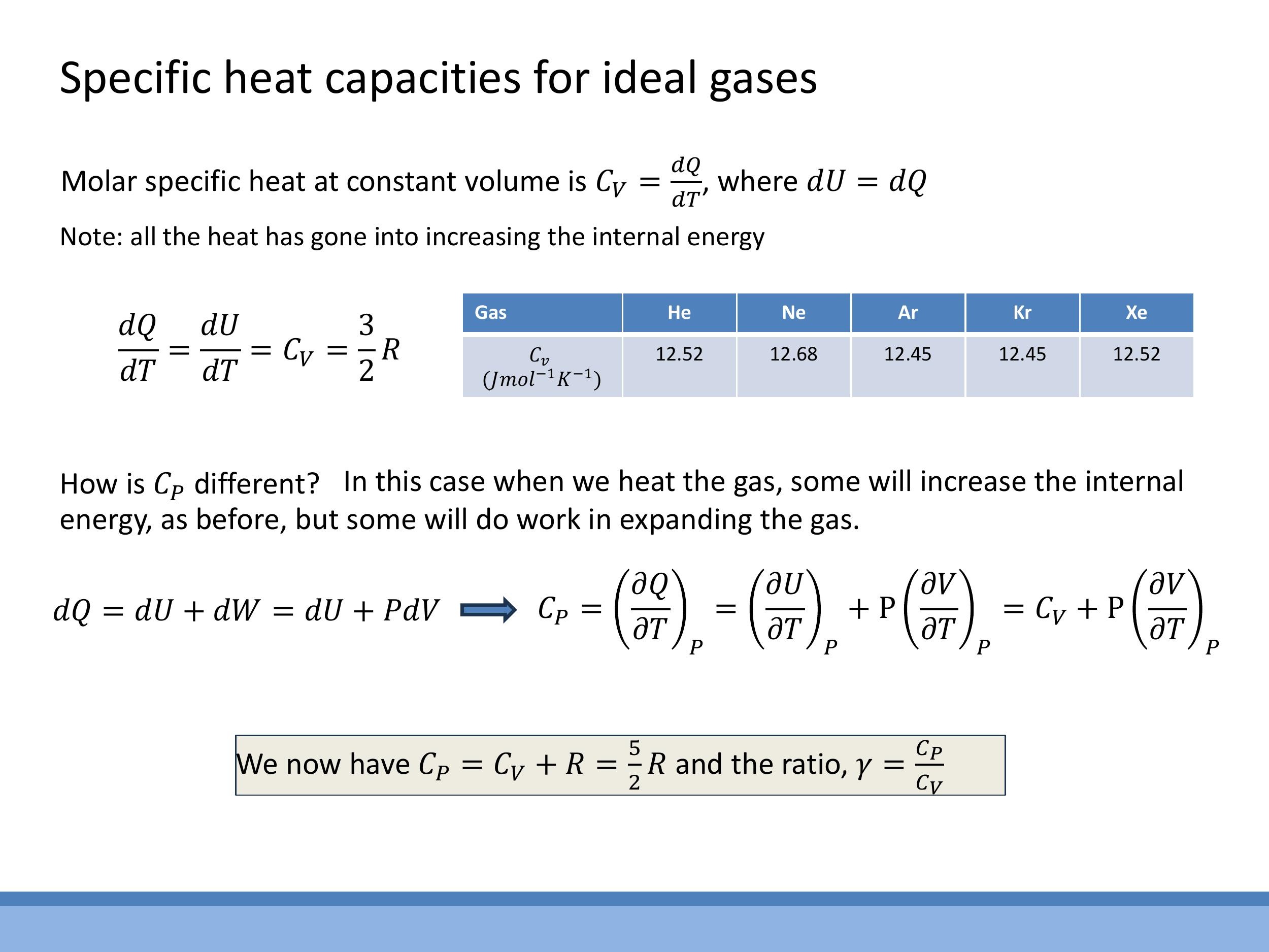
In the previous lecture, we discussed the specific heat capacities of ideal gases. We found that the equipartition theorem predicts a molar heat capacity of $\frac{1}{2}R$ for each quadratic degree of freedom. For a monatomic ideal gas, with its three translational degrees of freedom, this gives a specific heat at constant volume, $C_V = \frac{3}{2}R$. The specific heat at constant pressure, $C_P$, is related by Mayer's relation, $C_P = C_V + R$, which for a monatomic gas yields $C_P = \frac{5}{2}R$. The ratio of these, $\gamma = \frac{C_P}{C_V}$, is $\frac{5}{3}$ for monatomic gases. Experimental data for noble gases, such as Helium, Neon, and Argon, closely matches this theoretical value, confirming their near-ideal behaviour. Today, we'll explore why the ideal gas assumptions break down for real gases and how we modify our models to account for these deviations.
When tackling real gas formulas in assessments, you won't need to memorise complex derivations or specific numerical constants for different gases. Instead, you'll be provided with the necessary formulas and values. The focus will be on recognising the underlying physics, substituting the given values correctly, and calculating the result.
1) What breaks in the ideal gas model, and what does it change?
The ideal gas model simplifies reality by making two key assumptions that fail for real gases. Firstly, it assumes there are no intermolecular forces between particles. In truth, real molecules experience both attractive and steeply repulsive forces at close range. Secondly, the ideal gas model treats particles as point-like, possessing mass but no volume. In reality, atoms and molecules have a finite, non-zero size.
These failed idealisations have significant consequences for the macroscopic state variables of a gas. For pressure, the attractive intermolecular forces can subtly reduce the momentum transferred to the container walls during collisions. This means the measured pressure, $P$, can be lower than it would be if no attractions were present. For volume, the finite size of the molecules themselves reduces the actual 'free volume' available for other molecules to move in. Therefore, the total container volume, $V$, must be replaced by an effective available volume that is smaller than $V$.
2) Modelling real gases: van der Waals and the virial view
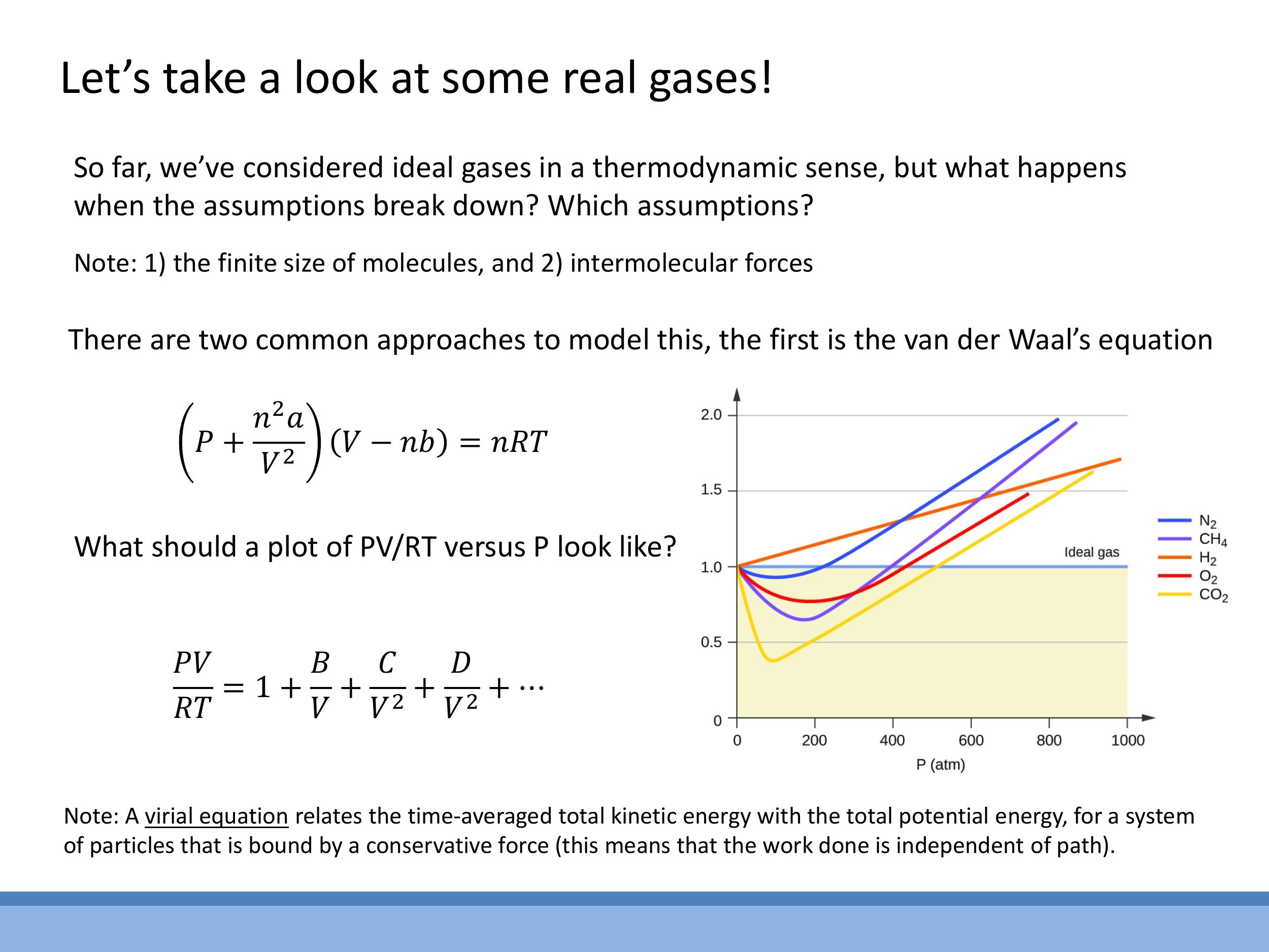
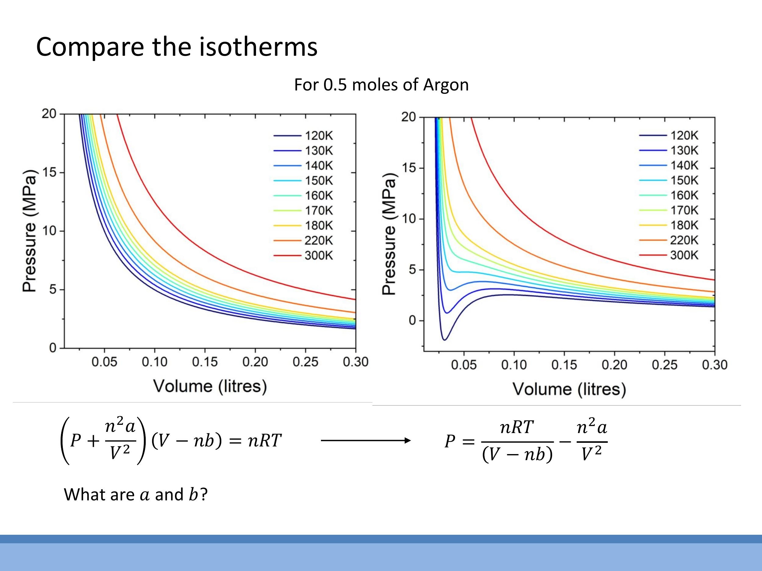
One of the most physically intuitive models for real gases is the van der Waals (vdW) equation. It introduces corrections to the ideal gas law to account for the finite size of molecules and intermolecular attractions. For $n$ moles of gas, the van der Waals equation is:
$$
\left( P + \frac{n^2 a}{V^2} \right) (V - nb) = nRT
$$
Here, the term $\frac{n^2 a}{V^2}$ corrects for intermolecular attraction (affecting the pressure term), and the term $nb$ corrects for the finite size of the molecules (reducing the available volume).
An alternative, more empirical approach is the virial equation, which expresses the deviation from ideal gas behaviour as a power series in inverse volume:
$$
\frac{PV}{RT} = 1 + \frac{B}{V} + \frac{C}{V^2} + \dots
$$
In this equation, the coefficients $B, C, \dots$ are determined by fitting the series to experimental data.
Experimental observations clearly show how real gases deviate from ideal behaviour. If we plot $\frac{PV}{RT}$ against pressure $P$ for one mole of gas, an ideal gas would show a constant value of 1. However, real gases deviate significantly from this ideal line at higher pressures and lower temperatures. Different gases exhibit different deviations, some dipping below 1 and others rising above it. Both the van der Waals equation and the virial equation recover the ideal gas law ($PV = nRT$) in the limit of low density (very large $V$) or high temperature, where intermolecular attractions become rare and the finite size of molecules becomes negligible.
3) Finite-size correction (b): the excluded volume
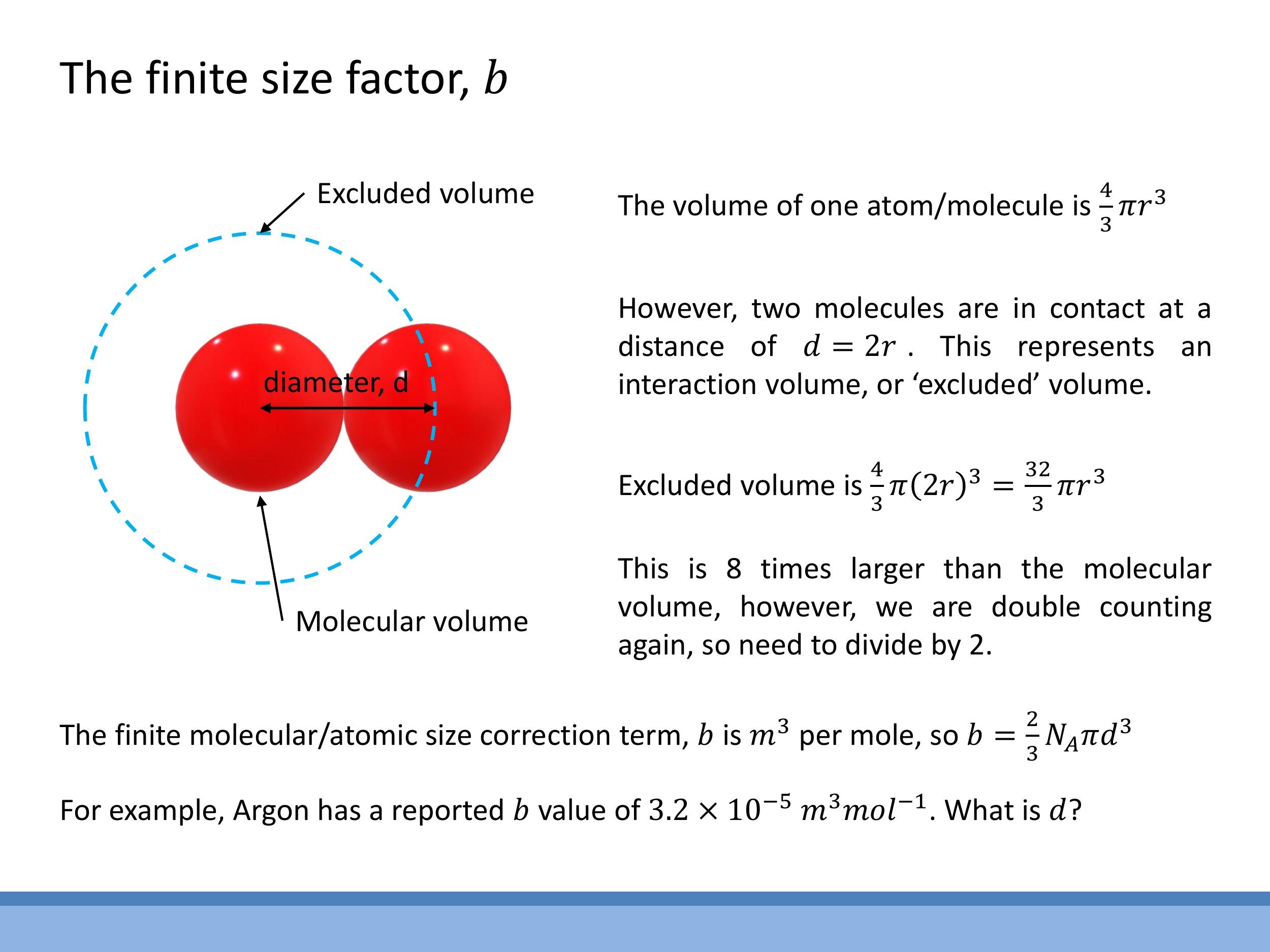
The correction term $b$ in the van der Waals equation accounts for the finite size of gas molecules, effectively reducing the available volume for motion. We can derive this term by picturing molecules as hard spheres of diameter $d$. When two such molecules are in contact, the centre of one molecule cannot enter a spherical region of radius $d$ around the centre of the other. This region represents an "excluded volume" that is unavailable for other molecules.
To calculate the excluded volume for a pair, we consider a sphere of radius $d$. Its volume is $\frac{4}{3}\pi d^3$. Since this excluded volume is shared between the two interacting molecules, we divide it by two to avoid double-counting. Therefore, the excluded volume per molecule is $\frac{1}{2} \times \frac{4}{3}\pi d^3 = \frac{2}{3}\pi d^3$. To find the molar correction $b$, we multiply this by Avogadro's number, $N_A$:
$$
b = \frac{2}{3} N_A \pi d^3
$$
The units of $b$ are $\text{m}^3 \, \text{mol}^{-1} $. For example, Argon has a $ b $ value of approximately $ 3.2 \times 10^{-5} \, \text{m}^3 \, \text{mol}^{-1} $. This value, though small, becomes significant at high densities. This derivation helps us understand the intuition behind replacing $ V $ with $ V - nb$, which represents the 'free volume' accessible to the gas molecules.
4) Attraction correction (a): why the wall pressure is lower
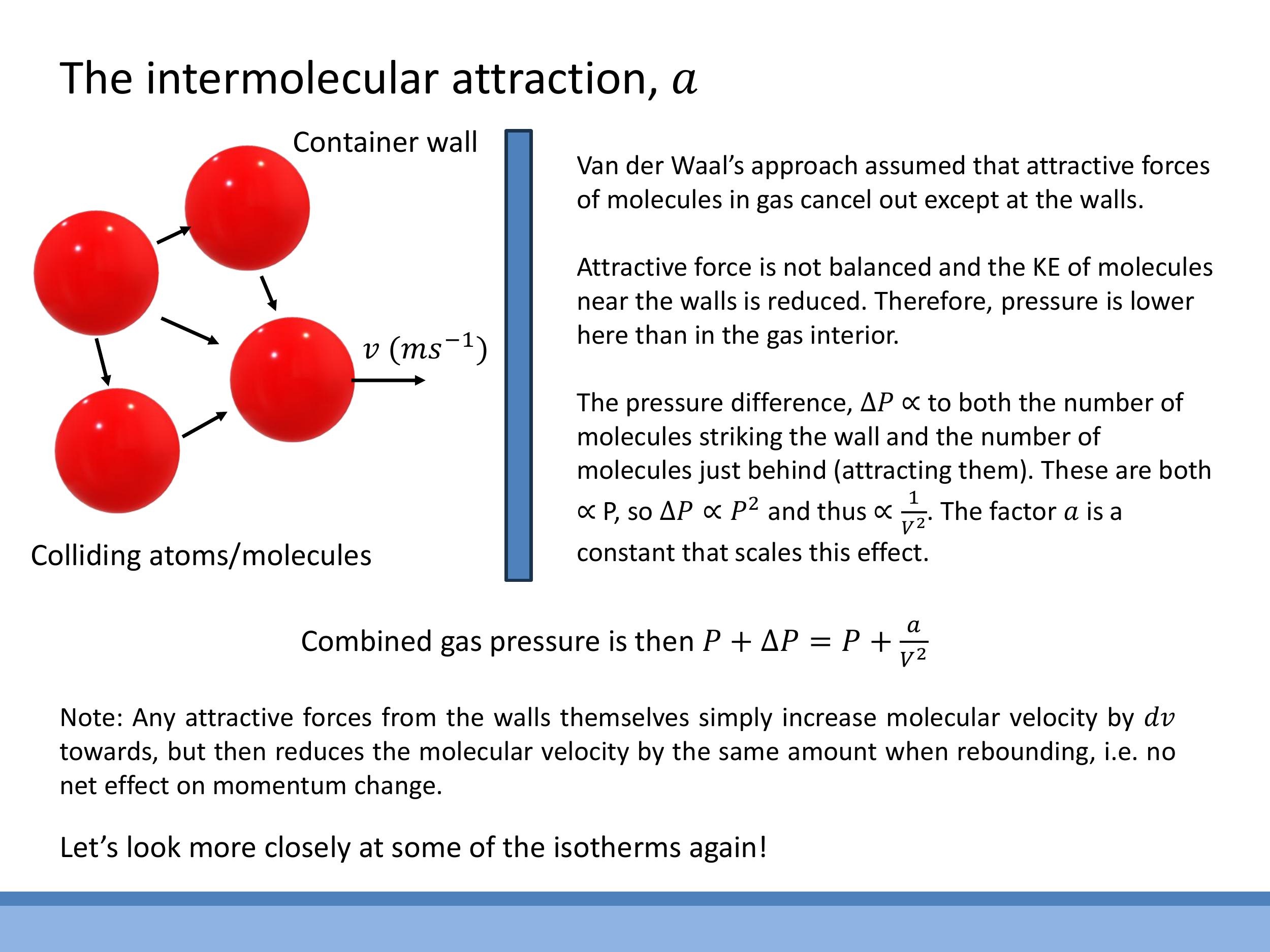
The correction term $a$ in the van der Waals equation accounts for the attractive intermolecular forces. Within the bulk of a gas, these attractive forces generally cancel out in all directions due to the symmetrical distribution of neighbouring molecules. However, this symmetry breaks down for molecules located near the container walls. Molecules close to a wall experience a net inward pull from the molecules behind them, as there are no molecules on the other side of the wall to exert an opposing pull.
This net inward force causes molecules to strike the wall with reduced momentum, leading to a lower measured pressure than the internal pressure within the gas. The magnitude of this pressure reduction, $\Delta P$, depends on two factors: the rate at which molecules collide with the wall (which is proportional to the number density, $n/V$), and the strength of the inward pull (which is also proportional to the number density, $n/V$). Consequently, the pressure reduction is proportional to the square of the number density: $\Delta P \propto (n/V)^2$. This is why the van der Waals equation modifies the pressure term by adding $a(n/V)^2$, where $a$ is a constant that scales the effect for a specific gas.
5) Reading P-V isotherms: ideal vs real, and what “loops” really mean
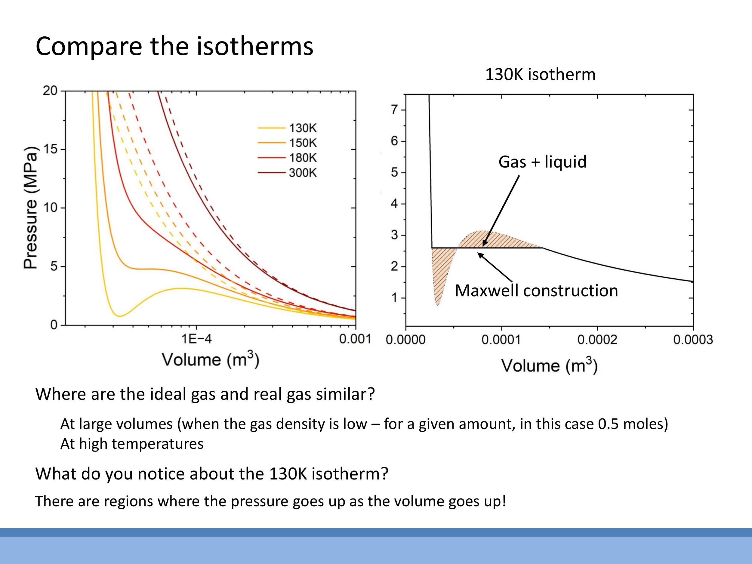
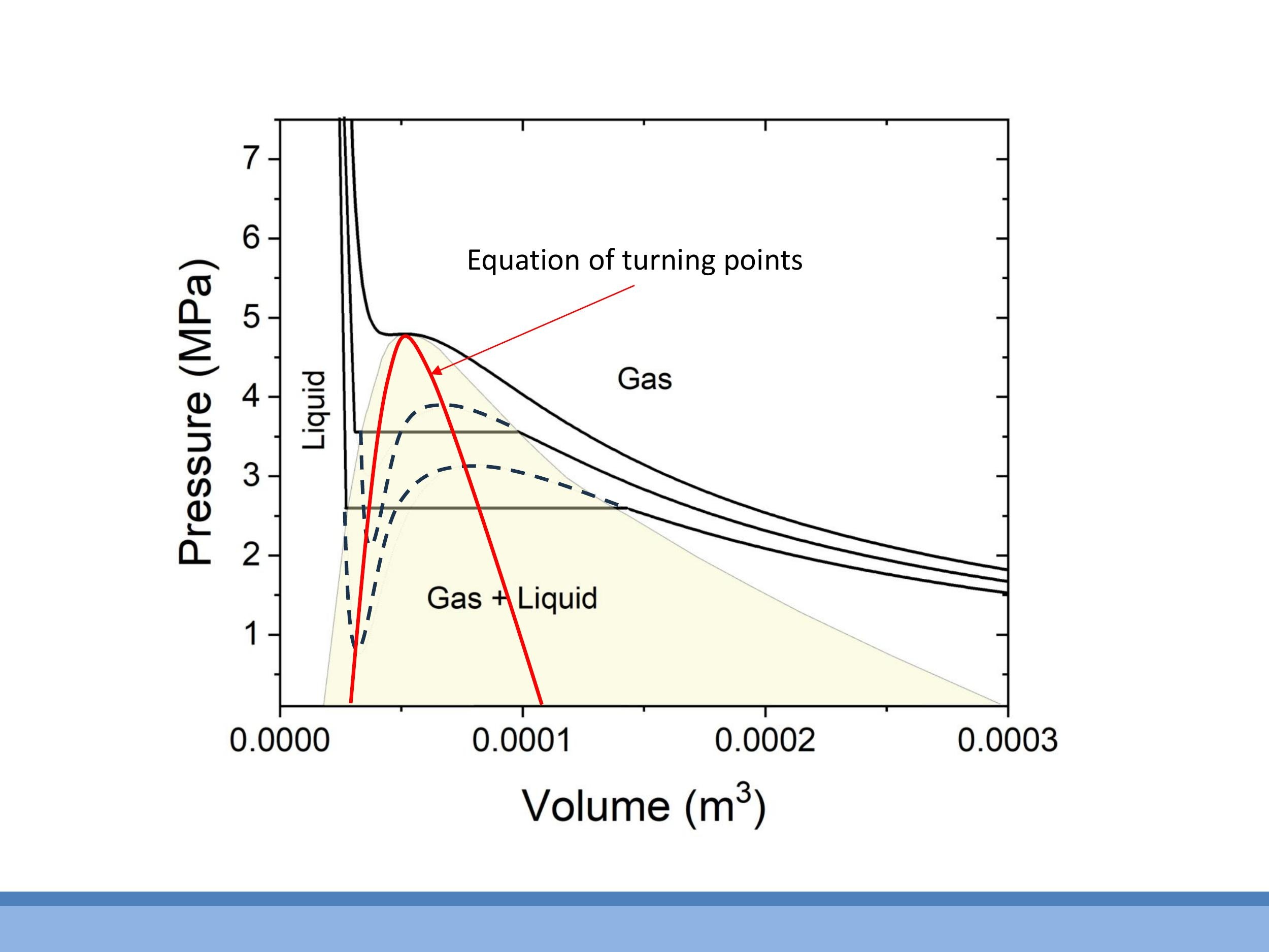
When we plot pressure-volume ($P-V$) isotherms, which show the relationship between pressure and volume at a constant temperature, we observe distinct differences between ideal and real gases. At high temperatures, real gas isotherms closely resemble the hyperbolic curves predicted by the ideal gas law. However, at lower temperatures, the van der Waals equation predicts a characteristic S-shaped loop in the isotherms. This loop includes regions where $\text{d}P/\text{d}V > 0$ (pressure increases with volume) or even where pressure is negative, which are physically impossible for a single, stable gas phase.
This unphysical loop actually signals a phase change: the gas is condensing into a liquid. The loop corresponds to a gas-liquid coexistence region. During compression at a fixed temperature in this region, the gas doesn't simply increase its pressure; instead, it converts into a liquid at a constant pressure. Once the substance is entirely liquid, further compression leads to a very steep rise in pressure for a small change in volume, reflecting the near-incompressibility of liquids.
To correct the unphysical loop, we use the Maxwell construction
6) The critical isotherm and the scale $T_C \sim \varepsilon/k$
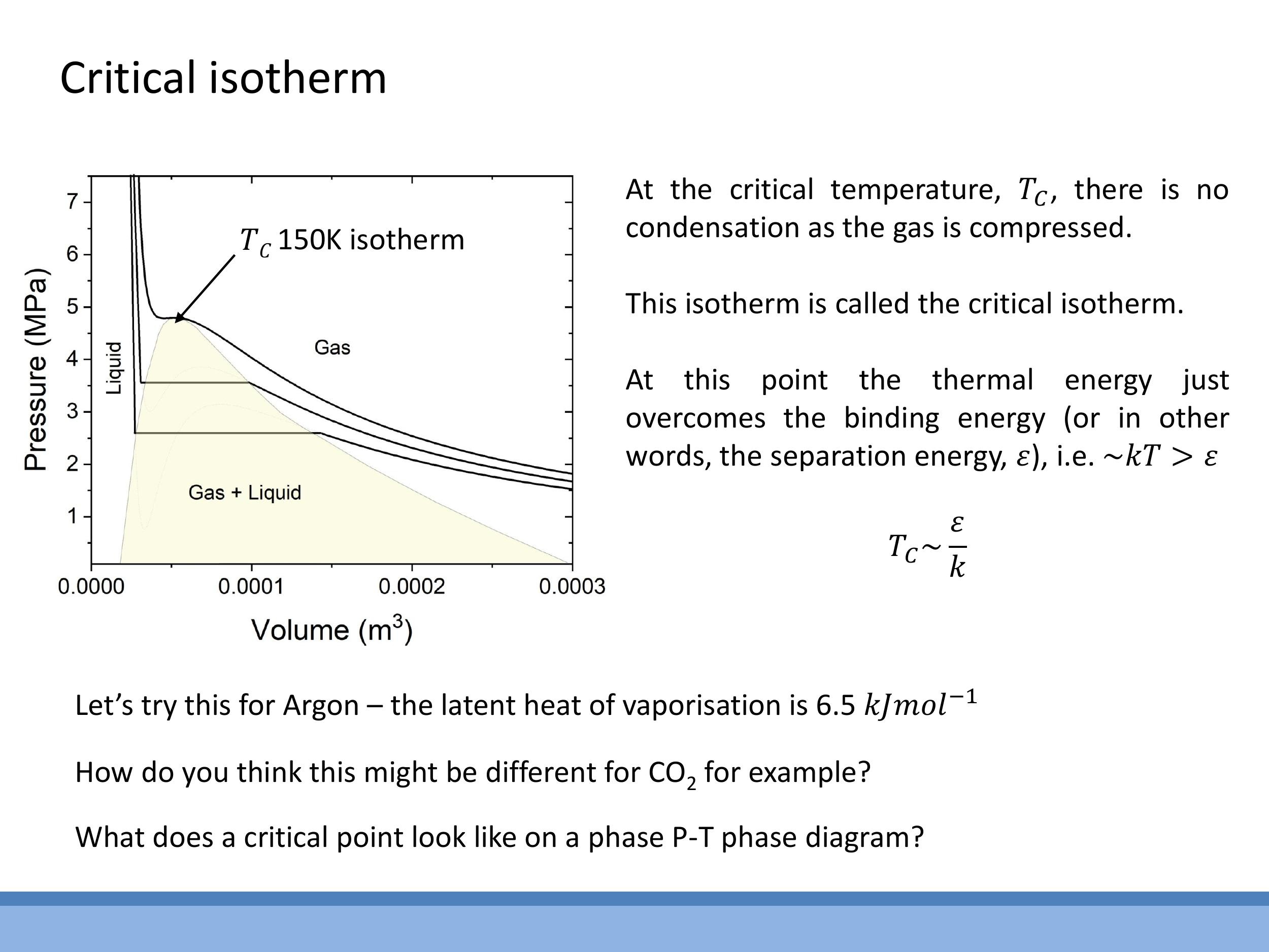
As the temperature of a gas increases, the S-shaped loop on the van der Waals isotherms shrinks. At a specific temperature, known as the critical temperature ($T_C$), the loop completely disappears. At this point, the isotherm exhibits a horizontal tangent at a single point of inflection, known as the critical point. Above $T_C$, compression alone cannot cause the gas to condense into a liquid; instead, it transitions smoothly into a dense fluid without a distinct phase boundary.
The critical temperature provides a crucial link between macroscopic and microscopic energy scales. At $T_C$, the average thermal energy, $kT$, is comparable to the intermolecular binding or separation energy, $\varepsilon$. This relationship allows us to estimate the critical temperature as $T_C \sim \frac{\varepsilon}{k}$. This connects back to earlier discussions where $\varepsilon$ was determined from latent heats and nearest-neighbour interactions, demonstrating how the same fundamental energy scale governs both microscopic bond strength and macroscopic phase transitions.
7) Phase diagrams: triple point, critical point, and supercritical fluids
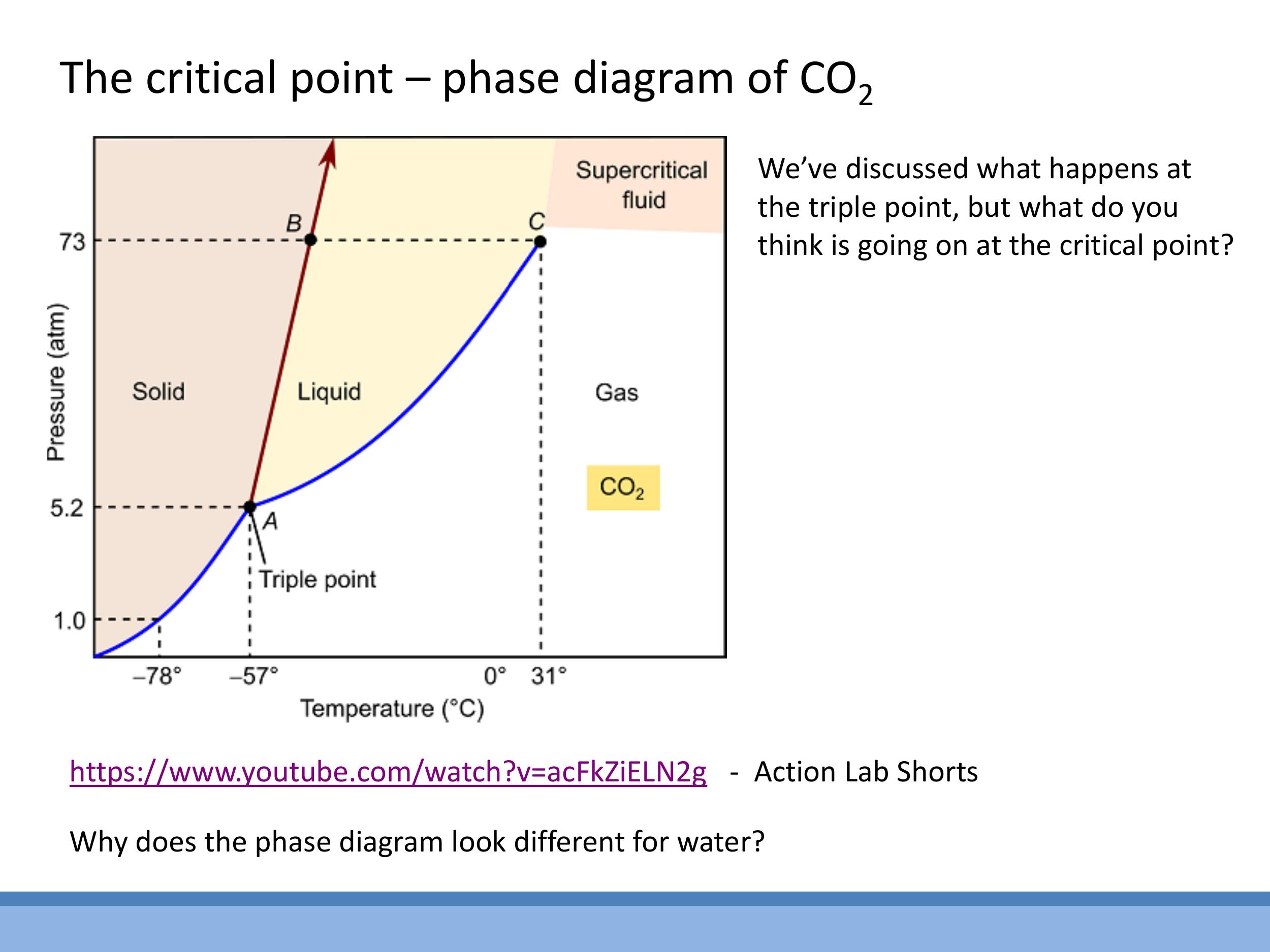
A pressure-temperature ($P-T$) phase diagram, such as that for carbon dioxide ($\text{CO}_2$), provides a comprehensive map of the different phases (solid, liquid, gas) and the boundaries between them. The lines on the diagram represent conditions where two phases coexist in equilibrium. The triple point is a unique pressure and temperature at which all three phases-solid, liquid, and gas-can coexist simultaneously in equilibrium. The critical point ($T_C, P_C$) marks the end of the liquid-gas phase boundary. Beyond this point, at temperatures and pressures above the critical point, the distinction between liquid and gas vanishes.
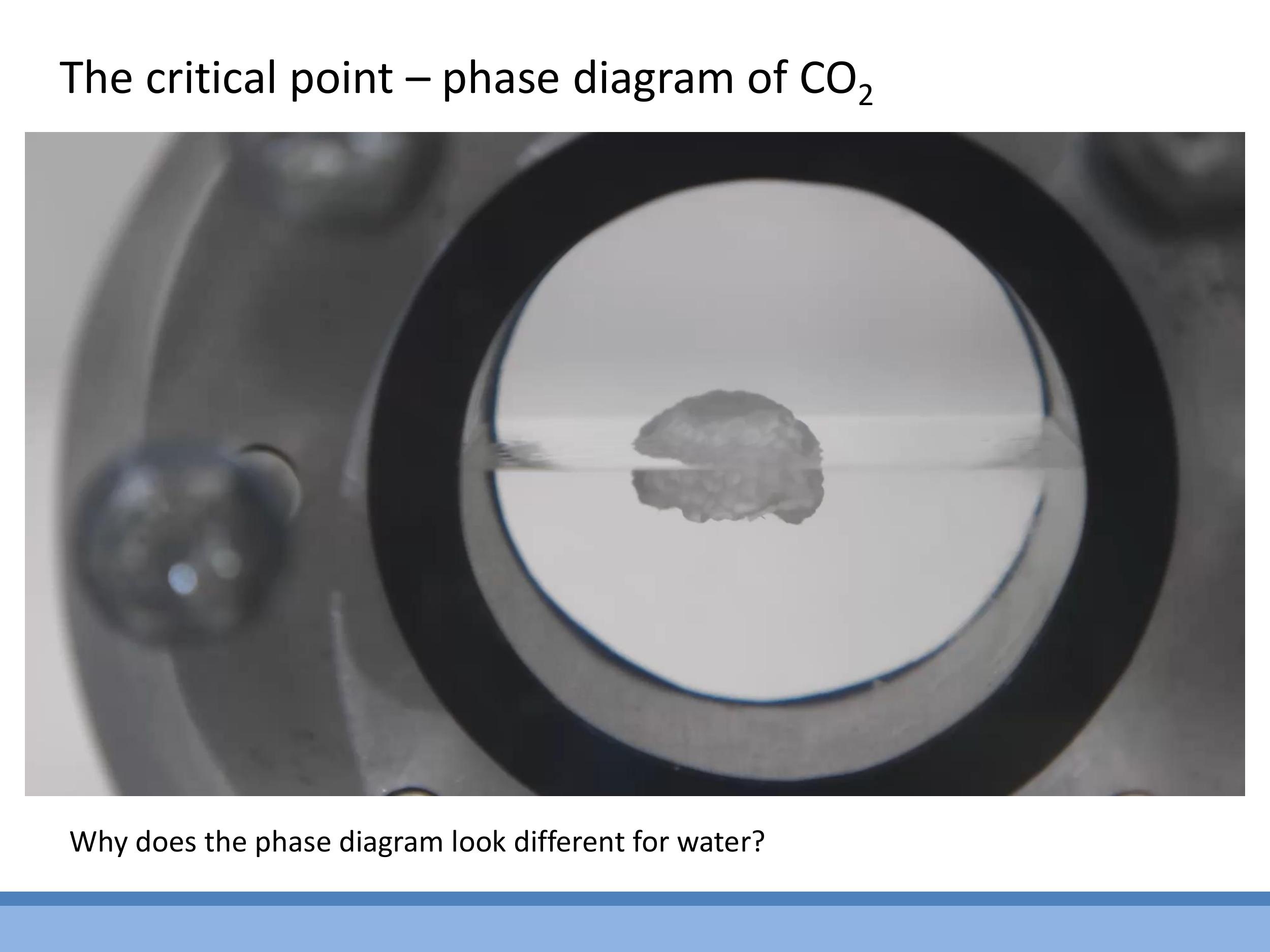
This region is known as the supercritical fluid state. A supercritical fluid behaves as a dense, viscous "liquidy gas" with properties intermediate between those of a liquid and a gas. For instance, in a demonstration with liquid $\text{CO}_2$, as it is gently heated to its critical temperature (around $31 \, ^\circ\text{C}$), the meniscus (the clear boundary between liquid and gas) gradually fades and disappears, indicating that the fluid has entered the supercritical state. An object floating at the interface would then sink, as the fluid becomes a uniform, dense medium.
Water, however, exhibits an anomalous phase diagram. Unlike most substances, for which the solid-liquid boundary line has a positive slope (meaning increasing pressure favours the denser solid phase), water's solid-liquid boundary has a negative slope. This unusual behaviour occurs because ice is less dense than liquid water. Consequently, increasing the pressure on ice at a near-constant temperature can cause it to melt, a phenomenon crucial for processes like ice skating and the survival of aquatic life in cold climates.
Appendix: Locating the critical point from the vdW isotherm (outline only)
Side Note: This material is supplementary and won't be examined, but provides useful context.
The critical point on a van der Waals isotherm can be determined mathematically. For a given temperature, the turning points of the isotherm, where $\text{d}P/\text{d}V = 0$, can be found. Since the van der Waals equation is cubic in $V$, it can have up to two such turning points (a local maximum and a local minimum). The critical point occurs when these two turning points merge into a single point of inflection. This happens when both $\text{d}P/\text{d}V = 0$ and $\text{d}^2P/\text{d}V^2 = 0$ simultaneously. Solving these two equations yields expressions for the critical volume ($V_C$), critical pressure ($P_C$), and critical temperature ($T_C$) in terms of the van der Waals constants $a$ and $b$. These derivations are typically explored in problems classes.
Key takeaways
Two ideal-gas assumptions fail for real gases: molecules are not point-like and they do interact via intermolecular forces. These failures lead to corrections in the van der Waals equation: the volume $V$ is replaced by $V - nb$, and the pressure $P$ is replaced by $P + a(n/V)^2$.
The finite-size correction term $b$ arises from the excluded volume of hard spheres. For one mole, it is given by $b = \frac{2}{3} N_A \pi d^3$, with units of $\text{m}^3 \, \text{mol}^{-1}$.
The attraction correction term $a$ accounts for the reduced pressure at the container walls. Molecules near a wall experience a net inward pull, causing them to hit the wall with less momentum. The resulting pressure reduction scales quadratically with the number density, $\Delta P \propto (n/V)^2$.
At low temperatures, van der Waals isotherms predict an S-shaped loop, which is physically resolved by the Maxwell construction. This construction replaces the loop with a constant-pressure plateau, representing the coexistence of gas and liquid. The steep region at small volumes reflects the near-incompressibility of liquids.
The critical isotherm, at temperature $T_C$, is where the loop vanishes. Above $T_C$, a gas cannot be liquefied by compression alone. Physically, $T_C$ is set by the energetic balance between thermal energy and intermolecular binding energy, $kT_C \sim \varepsilon$.
Pressure-temperature ($P-T$) phase diagrams summarise the phases and their boundaries. They show the triple point (where solid, liquid, and gas coexist) and the critical point (the end of the liquid-gas boundary), beyond which lies the supercritical region. Water is anomalous because its solid-liquid boundary has a negative slope, meaning ice is less dense than liquid water, allowing increased pressure to melt ice.
## Lecture 8: Real Gases
### 0) Orientation, quick review, and assessment guidance

In the previous lecture, we discussed the specific heat capacities of ideal gases. We found that the equipartition theorem predicts a molar heat capacity of $\frac{1}{2}R$ for each quadratic degree of freedom. For a monatomic ideal gas, with its three translational degrees of freedom, this gives a specific heat at constant volume, $C_V = \frac{3}{2}R$. The specific heat at constant pressure, $C_P$, is related by Mayer's relation, $C_P = C_V + R$, which for a monatomic gas yields $C_P = \frac{5}{2}R$. The ratio of these, $\gamma = \frac{C_P}{C_V}$, is $\frac{5}{3}$ for monatomic gases. Experimental data for noble gases, such as Helium, Neon, and Argon, closely matches this theoretical value, confirming their near-ideal behaviour. Today, we'll explore why the ideal gas assumptions break down for real gases and how we modify our models to account for these deviations.
When tackling real gas formulas in assessments, you won't need to memorise complex derivations or specific numerical constants for different gases. Instead, you'll be provided with the necessary formulas and values. The focus will be on recognising the underlying physics, substituting the given values correctly, and calculating the result.
### 1) What breaks in the ideal gas model, and what does it change?
The ideal gas model simplifies reality by making two key assumptions that fail for real gases. Firstly, it assumes there are no intermolecular forces between particles. In truth, real molecules experience both attractive and steeply repulsive forces at close range. Secondly, the ideal gas model treats particles as point-like, possessing mass but no volume. In reality, atoms and molecules have a finite, non-zero size.
These failed idealisations have significant consequences for the macroscopic state variables of a gas. For pressure, the attractive intermolecular forces can subtly reduce the momentum transferred to the container walls during collisions. This means the measured pressure, $P$, can be lower than it would be if no attractions were present. For volume, the finite size of the molecules themselves reduces the actual 'free volume' available for other molecules to move in. Therefore, the total container volume, $V$, must be replaced by an effective available volume that is smaller than $V$.
### 2) Modelling real gases: van der Waals and the virial view

One of the most physically intuitive models for real gases is the van der Waals (vdW) equation. It introduces corrections to the ideal gas law to account for the finite size of molecules and intermolecular attractions. For $n$ moles of gas, the van der Waals equation is:
$$ \left( P + \frac{n^2 a}{V^2} \right) (V - nb) = nRT $$
Here, the term $\frac{n^2 a}{V^2}$ corrects for intermolecular attraction (affecting the pressure term), and the term $nb$ corrects for the finite size of the molecules (reducing the available volume).
An alternative, more empirical approach is the virial equation, which expresses the deviation from ideal gas behaviour as a power series in inverse volume:
$$ \frac{PV}{RT} = 1 + \frac{B}{V} + \frac{C}{V^2} + \dots $$
In this equation, the coefficients $B, C, \dots$ are determined by fitting the series to experimental data.
Experimental observations clearly show how real gases deviate from ideal behaviour. If we plot $\frac{PV}{RT}$ against pressure $P$ for one mole of gas, an ideal gas would show a constant value of 1. However, real gases deviate significantly from this ideal line at higher pressures and lower temperatures. Different gases exhibit different deviations, some dipping below 1 and others rising above it. Both the van der Waals equation and the virial equation recover the ideal gas law ($PV = nRT$) in the limit of low density (very large $V$) or high temperature, where intermolecular attractions become rare and the finite size of molecules becomes negligible.
### 3) Finite-size correction (b): the excluded volume

The correction term $b$ in the van der Waals equation accounts for the finite size of gas molecules, effectively reducing the available volume for motion. We can derive this term by picturing molecules as hard spheres of diameter $d$. When two such molecules are in contact, the centre of one molecule cannot enter a spherical region of radius $d$ around the centre of the other. This region represents an "excluded volume" that is unavailable for other molecules.
To calculate the excluded volume for a pair, we consider a sphere of radius $d$. Its volume is $\frac{4}{3}\pi d^3$. Since this excluded volume is shared between the two interacting molecules, we divide it by two to avoid double-counting. Therefore, the excluded volume per molecule is $\frac{1}{2} \times \frac{4}{3}\pi d^3 = \frac{2}{3}\pi d^3$. To find the molar correction $b$, we multiply this by Avogadro's number, $N_A$:
$$ b = \frac{2}{3} N_A \pi d^3 $$
The units of $b$ are $\text{m}^3\,\text{mol}^{-1}$. For example, Argon has a $b$ value of approximately $3.2 \times 10^{-5}\,\text{m}^3\,\text{mol}^{-1}$. This value, though small, becomes significant at high densities. This derivation helps us understand the intuition behind replacing $V$ with $V - nb$, which represents the 'free volume' accessible to the gas molecules.
### 4) Attraction correction (a): why the wall pressure is lower

The correction term $a$ in the van der Waals equation accounts for the attractive intermolecular forces. Within the bulk of a gas, these attractive forces generally cancel out in all directions due to the symmetrical distribution of neighbouring molecules. However, this symmetry breaks down for molecules located near the container walls. Molecules close to a wall experience a net inward pull from the molecules behind them, as there are no molecules on the other side of the wall to exert an opposing pull.
This net inward force causes molecules to strike the wall with reduced momentum, leading to a lower measured pressure than the internal pressure within the gas. The magnitude of this pressure reduction, $\Delta P$, depends on two factors: the rate at which molecules collide with the wall (which is proportional to the number density, $n/V$), and the strength of the inward pull (which is also proportional to the number density, $n/V$). Consequently, the pressure reduction is proportional to the square of the number density: $\Delta P \propto (n/V)^2$. This is why the van der Waals equation modifies the pressure term by adding $a(n/V)^2$, where $a$ is a constant that scales the effect for a specific gas.
### 5) Reading P-V isotherms: ideal vs real, and what “loops” really mean


When we plot pressure-volume ($P-V$) isotherms, which show the relationship between pressure and volume at a constant temperature, we observe distinct differences between ideal and real gases. At high temperatures, real gas isotherms closely resemble the hyperbolic curves predicted by the ideal gas law. However, at lower temperatures, the van der Waals equation predicts a characteristic S-shaped loop in the isotherms. This loop includes regions where $\text{d}P/\text{d}V > 0$ (pressure increases with volume) or even where pressure is negative, which are physically impossible for a single, stable gas phase.
This unphysical loop actually signals a phase change: the gas is condensing into a liquid. The loop corresponds to a gas-liquid coexistence region. During compression at a fixed temperature in this region, the gas doesn't simply increase its pressure; instead, it converts into a liquid at a constant pressure. Once the substance is entirely liquid, further compression leads to a very steep rise in pressure for a small change in volume, reflecting the near-incompressibility of liquids.
To correct the unphysical loop, we use the **Maxwell construction**. This involves replacing the S-shaped region with a horizontal line, or plateau, at the constant pressure of the phase transition. This line is positioned such that the area enclosed by the loop above the line is equal to the area below it (the equal-area rule). This corrected isotherm accurately represents the different regions: the gas phase at large volumes, the gas + liquid coexistence phase along the flat plateau, and the liquid phase at small volumes with its characteristic steep pressure rise. The lower the temperature, the more pronounced the loop, indicating a stronger tendency for condensation, while higher temperatures "wash out" the loop, as thermal energy overcomes intermolecular attractions.
### 6) The critical isotherm and the scale $T_C \sim \varepsilon/k$

As the temperature of a gas increases, the S-shaped loop on the van der Waals isotherms shrinks. At a specific temperature, known as the **critical temperature ($T_C$)**, the loop completely disappears. At this point, the isotherm exhibits a horizontal tangent at a single point of inflection, known as the critical point. Above $T_C$, compression alone cannot cause the gas to condense into a liquid; instead, it transitions smoothly into a dense fluid without a distinct phase boundary.
The critical temperature provides a crucial link between macroscopic and microscopic energy scales. At $T_C$, the average thermal energy, $kT$, is comparable to the intermolecular binding or separation energy, $\varepsilon$. This relationship allows us to estimate the critical temperature as $T_C \sim \frac{\varepsilon}{k}$. This connects back to earlier discussions where $\varepsilon$ was determined from latent heats and nearest-neighbour interactions, demonstrating how the same fundamental energy scale governs both microscopic bond strength and macroscopic phase transitions.
### 7) Phase diagrams: triple point, critical point, and supercritical fluids


A pressure-temperature ($P-T$) phase diagram, such as that for carbon dioxide ($\text{CO}_2$), provides a comprehensive map of the different phases (solid, liquid, gas) and the boundaries between them. The lines on the diagram represent conditions where two phases coexist in equilibrium. The **triple point** is a unique pressure and temperature at which all three phases-solid, liquid, and gas-can coexist simultaneously in equilibrium. The **critical point** ($T_C, P_C$) marks the end of the liquid-gas phase boundary. Beyond this point, at temperatures and pressures above the critical point, the distinction between liquid and gas vanishes.
This region is known as the **supercritical fluid** state. A supercritical fluid behaves as a dense, viscous "liquidy gas" with properties intermediate between those of a liquid and a gas. For instance, in a demonstration with liquid $\text{CO}_2$, as it is gently heated to its critical temperature (around $31\,^\circ\text{C}$), the meniscus (the clear boundary between liquid and gas) gradually fades and disappears, indicating that the fluid has entered the supercritical state. An object floating at the interface would then sink, as the fluid becomes a uniform, dense medium.
Water, however, exhibits an anomalous phase diagram. Unlike most substances, for which the solid-liquid boundary line has a positive slope (meaning increasing pressure favours the denser solid phase), water's solid-liquid boundary has a negative slope. This unusual behaviour occurs because ice is less dense than liquid water. Consequently, increasing the pressure on ice at a near-constant temperature can cause it to melt, a phenomenon crucial for processes like ice skating and the survival of aquatic life in cold climates.
### Appendix: Locating the critical point from the vdW isotherm (outline only)

*Side Note:* This material is supplementary and won't be examined, but provides useful context.
The critical point on a van der Waals isotherm can be determined mathematically. For a given temperature, the turning points of the isotherm, where $\text{d}P/\text{d}V = 0$, can be found. Since the van der Waals equation is cubic in $V$, it can have up to two such turning points (a local maximum and a local minimum). The critical point occurs when these two turning points merge into a single point of inflection. This happens when both $\text{d}P/\text{d}V = 0$ and $\text{d}^2P/\text{d}V^2 = 0$ simultaneously. Solving these two equations yields expressions for the critical volume ($V_C$), critical pressure ($P_C$), and critical temperature ($T_C$) in terms of the van der Waals constants $a$ and $b$. These derivations are typically explored in problems classes.
## Key takeaways
Two ideal-gas assumptions fail for real gases: molecules are not point-like and they do interact via intermolecular forces. These failures lead to corrections in the van der Waals equation: the volume $V$ is replaced by $V - nb$, and the pressure $P$ is replaced by $P + a(n/V)^2$.
The finite-size correction term $b$ arises from the excluded volume of hard spheres. For one mole, it is given by $b = \frac{2}{3} N_A \pi d^3$, with units of $\text{m}^3\,\text{mol}^{-1}$.
The attraction correction term $a$ accounts for the reduced pressure at the container walls. Molecules near a wall experience a net inward pull, causing them to hit the wall with less momentum. The resulting pressure reduction scales quadratically with the number density, $\Delta P \propto (n/V)^2$.
At low temperatures, van der Waals isotherms predict an S-shaped loop, which is physically resolved by the Maxwell construction. This construction replaces the loop with a constant-pressure plateau, representing the coexistence of gas and liquid. The steep region at small volumes reflects the near-incompressibility of liquids.
The critical isotherm, at temperature $T_C$, is where the loop vanishes. Above $T_C$, a gas cannot be liquefied by compression alone. Physically, $T_C$ is set by the energetic balance between thermal energy and intermolecular binding energy, $kT_C \sim \varepsilon$.
Pressure-temperature ($P-T$) phase diagrams summarise the phases and their boundaries. They show the triple point (where solid, liquid, and gas coexist) and the critical point (the end of the liquid-gas boundary), beyond which lies the supercritical region. Water is anomalous because its solid-liquid boundary has a negative slope, meaning ice is less dense than liquid water, allowing increased pressure to melt ice.