Lecture 15: Elastic Solids - from stress-strain to atoms-on-springs
0) Orientation, admin, and bridge from crystals
This is the final lecture in the Properties of Matter course that introduces new material. Next week, a two-hour revision session will be held, covering both Mechanics and Properties of Matter. This session will replace Friday’s problems class, which has been cancelled. During the revision, the lecturer will highlight specific slides and topics that are particularly relevant for assessment.
In the previous lecture, we focused on the structure and packing of crystalline solids. Today, our goal is to bridge that understanding to how solids deform under external loads. We'll link the macroscopic elastic behaviour, such as stress, strain, and Young's modulus, to the underlying microscopic interatomic forces. The lecture will conclude by exploring entropy-driven elasticity, particularly in materials like rubber.
# 1) How solids respond to loads: types of stress and deformation
When an external force is applied to a solid, it experiences "stress," which is essentially the load distributed over a unit area. The material's response, or "deformation," depends on how this load is applied.
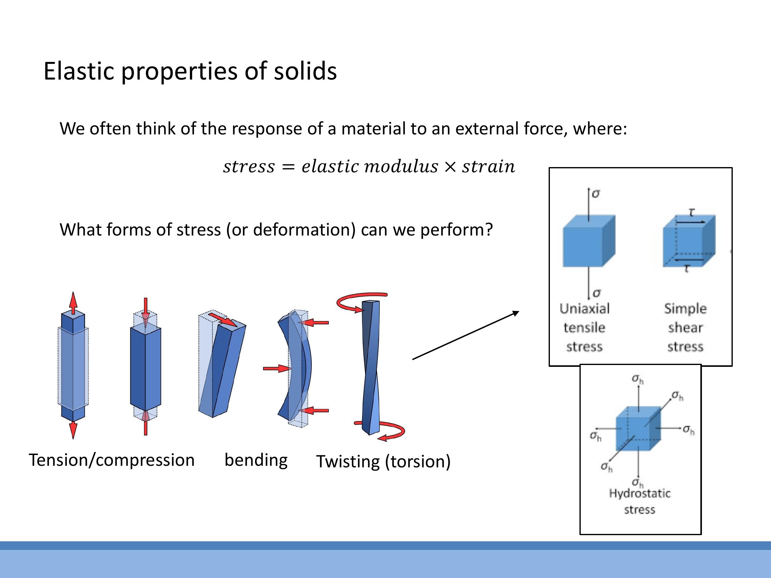
In practical applications, various forms of loading are used:
- Tension/Compression: This involves stretching or squashing a material along a single axis.
- Bending: An example is the three-point bend setup, which you encountered in your formative laboratory experiment, where a force is applied to the middle of a supported beam.
- Twisting (Torsion): This involves applying a torque about an axis, causing the material to twist.
- Hydrostatic Stress: This is a uniform compression applied from all directions, such as that experienced by materials in high-pressure cells.
# 2) Stress, strain, and Young’s modulus: the linear elastic regime
When a material is subjected to a tensile load, we define its response using specific quantities. Tensile stress, denoted by $\sigma$, is the force $F$ applied perpendicular to a cross-sectional area $A$:
$$
\sigma = \frac{F}{A}
$$
Tensile strain, $\varepsilon$, is the fractional change in length, $\Delta l$, relative to the original length $l$:
$$
\varepsilon = \frac{\Delta l}{l}
$$
In the initial, linear region of a material's stress-strain curve, stress is directly proportional to strain. The constant of proportionality is known as Young's modulus $E$, which quantifies the material's stiffness:
$$
E = \frac{\sigma}{\varepsilon}
$$
By substituting the definitions of stress and strain, this equation can be rearranged to resemble Hooke's law:
$$
F = \left( \frac{AE}{l} \right) \Delta l
$$
Here, the term $\left( \frac{AE}{l} \right)$ acts as an effective spring constant, $k_{\text{eff}}$. This analogy highlights the "springiness" of a material bar, showing how its inherent stiffness $E$, cross-sectional area $A$, and length $l$ combine to determine its resistance to stretching.
# 3) Reading a stress-strain curve: elastic limit, yield, hardening, necking, fracture
The stress-strain curve provides a comprehensive overview of a material's mechanical behaviour under increasing load.
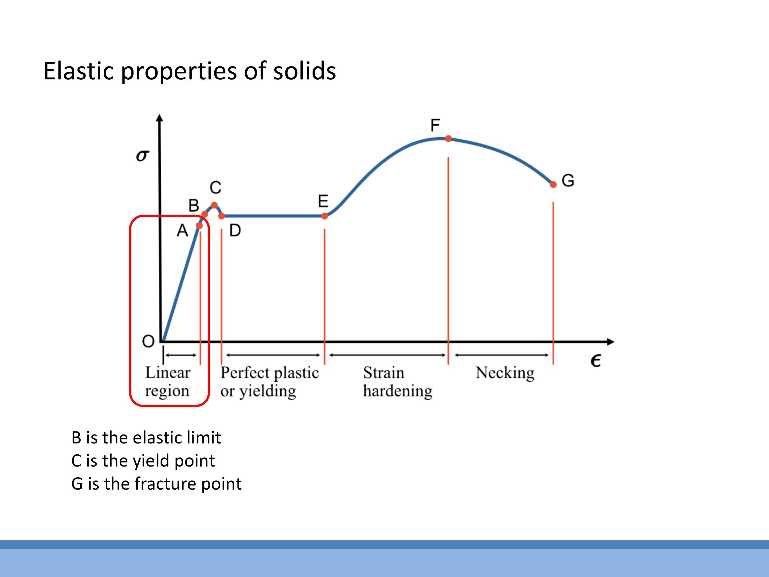
Starting from the origin:
- Linear elastic region: In this initial phase, stress is directly proportional to strain, with Young's modulus $E$ as the slope. If the load is removed, the material returns to its original length.
- Elastic limit B and yield point C: Beyond point B, the material ceases to behave purely elastically. The yield point C marks the onset of plastic deformation, where permanent changes in shape begin to occur.
- Plastic deformation: Microscopically, this involves the movement of defects called dislocations within the crystal lattice, allowing atomic planes to slip past one another.
- Strain (work) hardening: As deformation continues (towards point F), the material often becomes stiffer and harder. This "work hardening" occurs as dislocations accumulate and impede further slip, increasing resistance to deformation. A common example is bending a copper wire once, which makes it noticeably harder and more brittle if you try to bend it a second time. Tungsten wire, after one bend, can become so work-hardened that it shatters like glass on a second attempt.
- Necking and fracture (F → G): In the final stages of tensile loading, the material begins to thin locally, a phenomenon known as necking. This local thinning concentrates stress, ultimately leading to the material's fracture at point G.
# 4) Quantitative elasticity: extensions and stored energy
4.1 Extensions under load: order-of-magnitude checks
Understanding the quantitative aspects of elasticity allows us to predict how much a material will stretch under a given load. The rearranged Hooke's law form, $\Delta l = \frac{Fl}{AE}$, is crucial for these calculations.
Consider a practical example: a ~4.5 metre copper wire with a diameter of $120 \, \mu\text{m} $. If loads between $ 50 \, \text{g} $ and $ 150 \, \text{g} $ are applied, the extensions observed are typically of the order of $ 1 \, \text{mm}$ per added load, while the wire remains within its elastic limit. This matches our calculations, demonstrating that the model provides reasonable, physically sensible results.
Let's consider another example: a $1500 \, \text{kg} $ car suspended on a $ 2 \, \text{m} $ long steel cable with a diameter of $ 10 \, \text{mm} $. Steel has a Young's modulus of approximately $ 200 \, \text{GPa} $. Using the formula $ \Delta l = \frac{Fl}{AE} $, the extension for this setup is only a few millimetres, specifically around $ 2 \, \text{mm}$. This illustrates the strength of steel and the relatively small deformations experienced even under significant loads.
⚠️ Exam Alert! The lecturer explicitly stated: "This is not so different to the kind of questions you get in the multiple choice exam. In fact, this resembles one from last year, I think." You should be comfortable setting up and solving problems involving the extension of materials under load, similar to the car-on-cable example, ensuring your answer's magnitude is physically reasonable.
4.2 Energy stored in elastic extension
When a material is stretched within its elastic limit, the work done in deforming it is stored as elastic potential energy within its atomic bonds. This energy can be calculated by integrating the force with respect to the extension.
Starting with the force $F = \left( \frac{AE}{l} \right) \Delta l$, the work $W$ done to extend the material by $\Delta l$ is:
$$
W = \int F \, d(\Delta l) = \int_0^{\Delta l} \left( \frac{AE}{l} \right) \Delta l' \, d(\Delta l') = \frac{AE}{2l} (\Delta l)^2
$$
For the car-on-steel-cable example, where the extension was approximately $2 \, \text{mm} $, the stored elastic energy would be around $ 23 \, \text{J}$. This energy physically resides in the stretched bonds between the atoms.
⚠️ Exam Alert! The lecturer explicitly stated: "This sort of question is precisely what appeared in last year's multiple choice exam." You should be prepared to compute the stored elastic energy given the extension and material dimensions.
4.3 Live demo narrative: spotting the yield point with a copper wire
A live demonstration using a long, thin copper wire suspended with weights illustrates the concepts of elastic and plastic deformation. Initially, as the first two $50 \, \text{g} $ weights are added, the wire visibly extends by approximately $ 1.5 \, \text{mm} $ to $ 2 \, \text{mm}$ per step. In this elastic region, if the weights were removed, the wire would return to its original length.
However, once the total load reaches a certain point, typically around $150 \, \text{g} $ to $ 200 \, \text{g}$ for this wire, a critical change occurs. As further weights are added, the wire begins to stretch continuously and rapidly. This indicates that the yield strength of the copper has been exceeded, and plastic deformation has begun. When these larger loads are subsequently removed, the wire does not return to its initial length, confirming that it has undergone permanent deformation.
We can estimate the yield strength for copper, which is typically in the range of tens of megapascals. By using the relationship $\sigma_y \approx F_y/A$, where $F_y$ is the force at yield and $A$ is the wire's cross-sectional area, we can calculate the maximum "safe" load before the wire starts to plastically deform. This provides a practical sense of the material's limits. Microscopically, elastic deformation involves the reversible stretching of atomic bonds. Beyond the yield point, however, dislocations within the crystal lattice begin to move, causing atomic planes to slip past each other, resulting in a permanent change in the material's shape. This process can also lead to subsequent work hardening, where the material becomes stiffer due to the accumulation of these defects.
# 5) From atoms to E: deriving Young’s modulus from the interatomic potential
To understand the fundamental origin of a material's stiffness, we can connect the macroscopic Young's modulus directly to the microscopic interatomic potential. This approach builds upon the "atoms-on-springs" idea introduced earlier in the course.
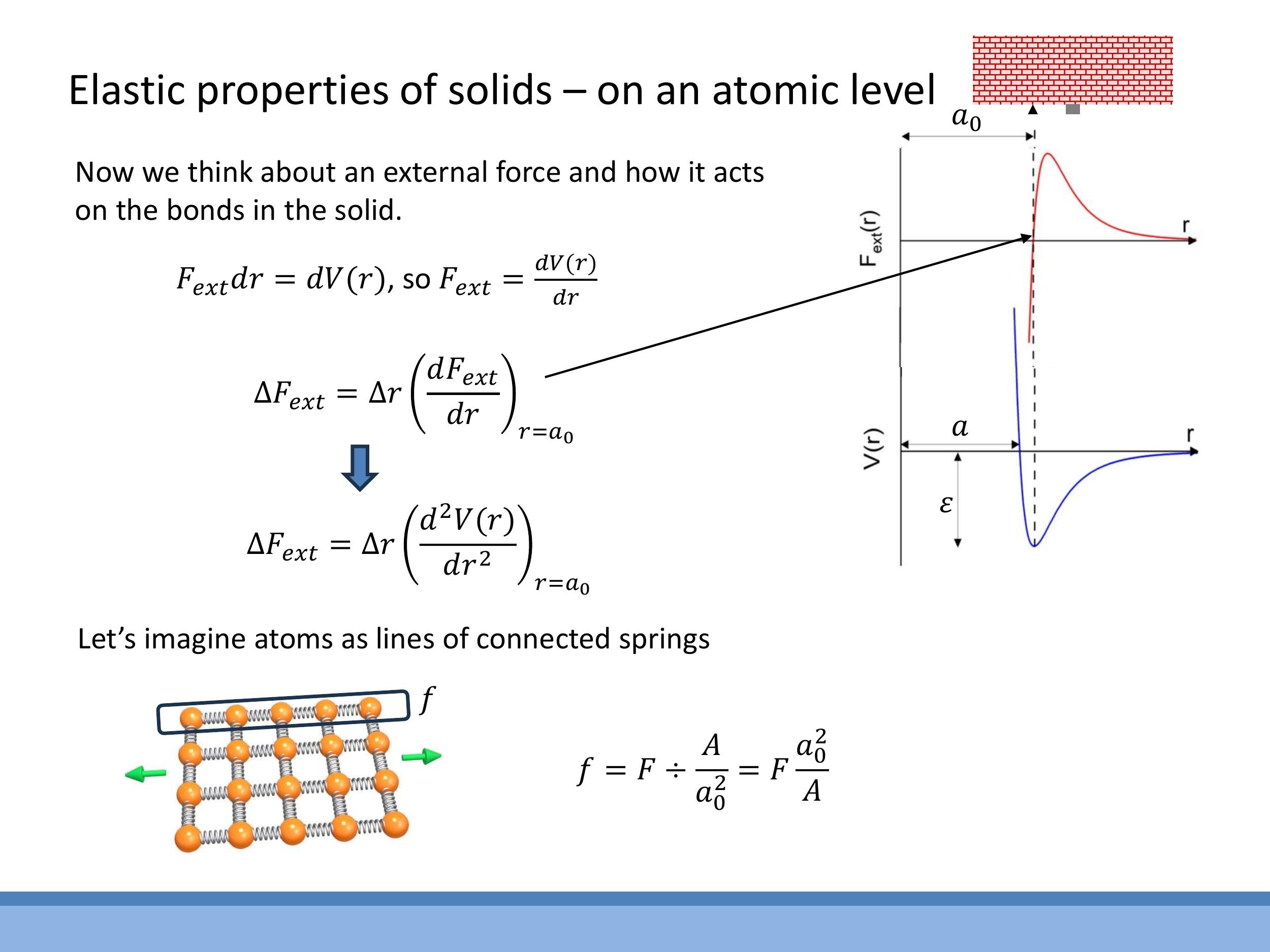
We begin by recalling the interatomic potential well, $V(r)$, which describes the energy of interaction between two atoms as a function of their separation $r$. This potential has a minimum at the equilibrium separation distance, $a_0$, and a well depth, $\varepsilon$, representing the bond energy. The force between atoms is given by the derivative of the potential, $F = dV/dr$.
For small displacements, $\Delta r$, around the equilibrium separation $a_0$, the force on a single bond can be approximated by linearising the force-distance curve:
$$\Delta F \approx \Delta r \left( \frac{dF}{dr} \right) {r=a_0} = \Delta r \left( \frac{d^2V}{dr^2} \right) {r=a_0} $$
This expression, $\left( \frac{d^2V}{dr^2} \right)_{r=a_0}$, represents the effective "spring constant" for a single interatomic bond.
To bridge the gap from microscopic bond forces to macroscopic Young's modulus, we relate the force per bond to the macroscopic force and the bond extension to the macroscopic extension:
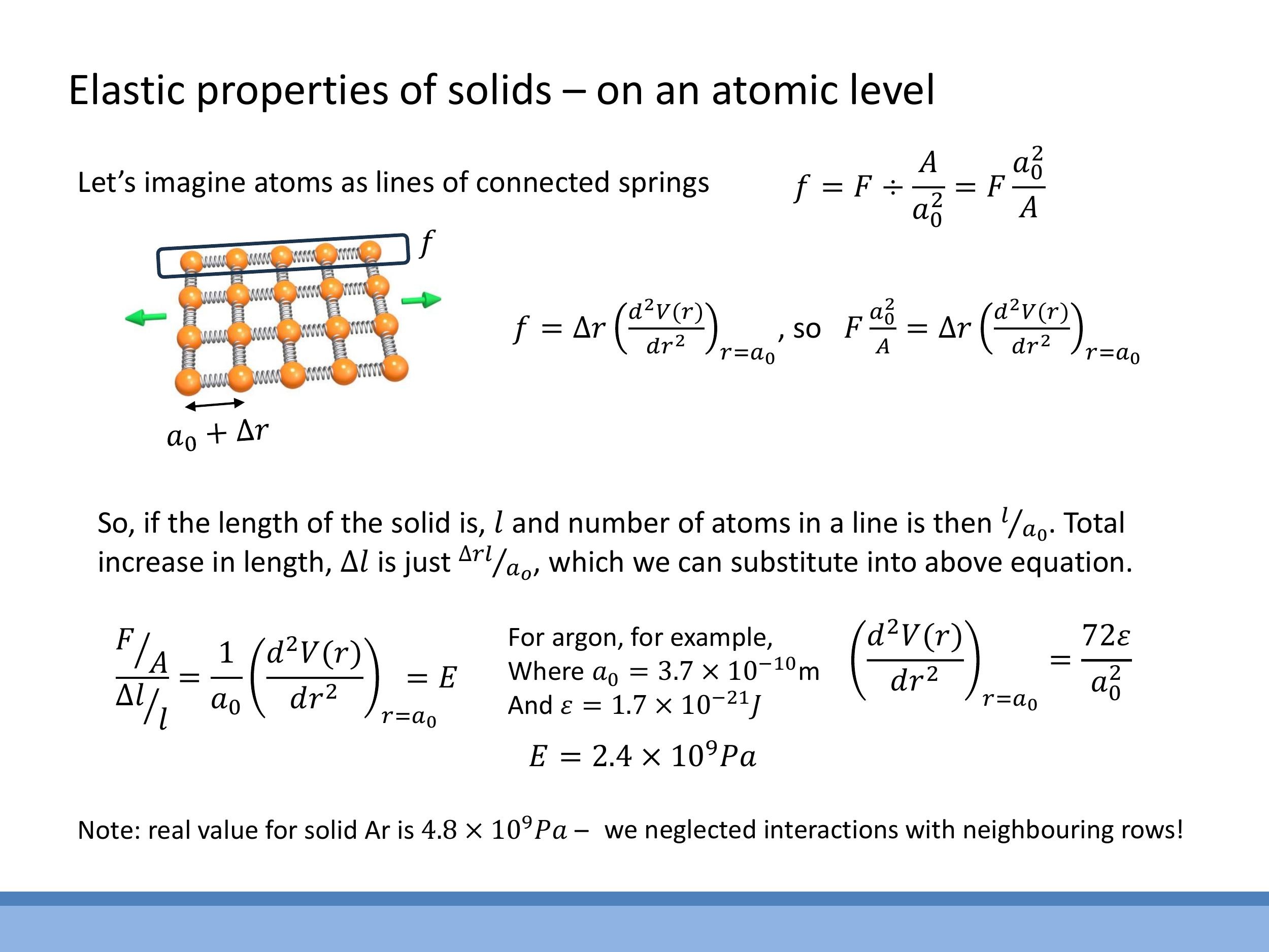
- The force per bond, $f$, can be related to the macroscopic force $F$ and the cross-sectional area $A$ by considering the density of bonds across that area. For a simple square lattice, this is approximately $f = F (a_0^2/A)$.
- The macroscopic total extension, $\Delta l$, of a wire of length $l$ is related to the extension of individual bonds, $\Delta r$, by the number of bonds in series along its length: $\Delta l = (l/a_0) \Delta r$.
Substituting these relationships into the definition of Young's modulus, $E = (F/A) / (\Delta l/l)$, leads to a powerful microscopic expression for $E$:
$$
E = \frac{1}{a_0} \left( \frac{d^2V}{dr^2} \right)_{r=a_0}
$$
This equation shows that Young's modulus is directly proportional to the curvature of the interatomic potential at its equilibrium minimum and inversely proportional to the equilibrium separation. A deeper, sharper potential well (higher $\frac{d^2V}{dr^2}$) indicates a stiffer material.
As a worked example, consider solid argon, which can be modelled using a Lennard-Jones potential. The second derivative of this potential at equilibrium is known to be $\left( \frac{d^2V}{dr^2} \right)_{r=a_0} = \frac{72\varepsilon}{a_0^2}$. Substituting this into our derived formula for $E$ gives:
$$
E = \frac{72\varepsilon}{a_0^3}
$$
Using typical values for solid argon, $a_0 \approx 3.7 \times 10^{-10} \, \text{m} $ and $ \varepsilon \approx 1.7 \times 10^{-21} \, \text{J} $, we calculate a Young's modulus of approximately $ 2.4 \, \text{GPa} $. The measured value for solid argon is closer to $ 4.8 \, \text{GPa}$. While our simple "independent chains" model is a factor of two off, it provides the correct order of magnitude and is a remarkably good approximation, with the discrepancy arising from neglecting the lateral coupling and interactions between neighbouring rows of atoms.
# 6) Entropic elasticity: why rubber heats when stretched and contracts when heated
Unlike metals, the elasticity of rubber is primarily driven by entropy rather than the stretching of individual bonds. This phenomenon, often called entropic elasticity, explains several counter-intuitive behaviours of rubber.
Microscopically, rubber consists of long, flexible polymer chains. In their natural, relaxed state, these chains are highly tangled and disordered, representing a state of high entropy. When a rubber band is stretched, these polymer chains are forced to align, resulting in a more ordered, lower-entropy configuration.
This change in entropy explains the elastocaloric effect, which you can feel by rapidly stretching a rubber band. When stretched suddenly, the band warms up. This is because stretching reduces the rubber's entropy. To comply with the Second Law of Thermodynamics (which states that the total entropy of the universe must increase or remain constant), the system must expel heat to its surroundings, increasing the entropy of the surroundings. This expelled heat is what you feel as warmth. Conversely, when the stretched band is released quickly, it contracts and cools. The chains spontaneously return to their higher-entropy, tangled state, absorbing heat from the surroundings to facilitate this increase in disorder.
A striking demonstration of entropic elasticity involves heating a hanging rubber band. While a metal wire would expand and lengthen when heated, a rubber band behaves differently. When a weighted rubber band is heated, it contracts and lifts the weight. This occurs because heating provides the polymer chains with enough thermal energy to explore a greater number of their accessible microstates, driving them towards their preferred, more disordered (higher-entropy) crumpled configurations. This increase in molecular chaos causes the band to shorten, contrasting sharply with the thermal expansion seen in most other materials.
# 7) Consolidation and next steps
This lecture has tied together macroscopic observations and microscopic models to explain the elastic properties of solids.
We began by defining macroscopic quantities like stress ($\sigma$), strain ($\varepsilon$), and Young's modulus ($E$), and then analysed the stress-strain curve, identifying key regions such as the elastic limit, plastic deformation, strain hardening, necking, and eventual fracture. We developed quantitative tools to calculate extensions ($\Delta l = \frac{Fl}{AE}$) and stored elastic energy ($W = \frac{AE}{2l} (\Delta l)^2$), emphasising the importance of order-of-magnitude checks for physical reasonableness.
From a microscopic perspective, we derived Young's modulus from the curvature of the interatomic potential $V(r)$ at the equilibrium separation $a_0$, showing that the "atoms-as-springs" model provides a powerful first approximation. Finally, we explored the thermodynamic link of entropic elasticity, explaining why rubber heats up when stretched and contracts when heated, a phenomenon governed by the polymer chains' preference for a disordered, high-entropy state.
Next week, a two-hour revision session will cover all material from both the Mechanics and Properties of Matter components of the course. The lecturer will highlight key slides and topics to help you prepare for the upcoming assessment.
Key takeaways
- Stress-strain relationships: Stress ($\sigma$) is defined as $F/A$, and strain ($\varepsilon$) as $\Delta l/l$. In the elastic region, stress is proportional to strain, with Young's modulus ($E$) as the constant of proportionality. Beyond the elastic limit, plastic deformation occurs due to dislocation motion, followed by strain hardening, necking, and ultimately fracture.
- Elastic behaviour: A material bar under tension can be modelled as a spring with an effective spring constant $k_{\text{eff}} = AE/l$. Extensions ($\Delta l = \frac{Fl}{AE}$) are typically in the millimetre range for metre-scale metal objects under common loads.
- Stored elastic energy: The work done in stretching a material is stored as elastic potential energy, given by $W = \frac{AE}{2l} (\Delta l)^2$.
- Microscopic origin of stiffness: Young's modulus can be derived from the interatomic potential, $V(r)$, as $E = \frac{1}{a_0} \left( \frac{d^2V}{dr^2} \right)_{r=a_0}$. For Lennard-Jones solids like argon, this model provides the correct order of magnitude, with small discrepancies explained by neglecting lateral interactions between atomic rows.
- Entropic elasticity: Rubber's unique elastic properties are driven by entropy. Stretching aligns polymer chains, reducing their entropy and causing heat expulsion. Conversely, heating a stretched rubber band increases the chains' disorder (entropy), causing the band to contract.
- Administrative: This marks the final lecture with new course content. A two-hour revision session for both Mechanics and Properties of Matter will replace the cancelled problems class and will focus on exam-relevant material.
## Lecture 15: Elastic Solids - from stress-strain to atoms-on-springs
### 0) Orientation, admin, and bridge from crystals
This is the final lecture in the Properties of Matter course that introduces new material. Next week, a two-hour revision session will be held, covering both Mechanics and Properties of Matter. This session will replace Friday’s problems class, which has been cancelled. During the revision, the lecturer will highlight specific slides and topics that are particularly relevant for assessment.
In the previous lecture, we focused on the structure and packing of crystalline solids. Today, our goal is to bridge that understanding to how solids deform under external loads. We'll link the macroscopic elastic behaviour, such as stress, strain, and Young's modulus, to the underlying microscopic interatomic forces. The lecture will conclude by exploring entropy-driven elasticity, particularly in materials like rubber.
## # 1) How solids respond to loads: types of stress and deformation
When an external force is applied to a solid, it experiences "stress," which is essentially the load distributed over a unit area. The material's response, or "deformation," depends on how this load is applied.

In practical applications, various forms of loading are used:
* **Tension/Compression:** This involves stretching or squashing a material along a single axis.
* **Bending:** An example is the three-point bend setup, which you encountered in your formative laboratory experiment, where a force is applied to the middle of a supported beam.
* **Twisting (Torsion):** This involves applying a torque about an axis, causing the material to twist.
* **Hydrostatic Stress:** This is a uniform compression applied from all directions, such as that experienced by materials in high-pressure cells.
## # 2) Stress, strain, and Young’s modulus: the linear elastic regime
When a material is subjected to a tensile load, we define its response using specific quantities. Tensile stress, denoted by $\sigma$, is the force $F$ applied perpendicular to a cross-sectional area $A$:
$$\sigma = \frac{F}{A}$$
Tensile strain, $\varepsilon$, is the fractional change in length, $\Delta l$, relative to the original length $l$:
$$\varepsilon = \frac{\Delta l}{l}$$
In the initial, linear region of a material's stress-strain curve, stress is directly proportional to strain. The constant of proportionality is known as Young's modulus $E$, which quantifies the material's stiffness:
$$E = \frac{\sigma}{\varepsilon}$$
By substituting the definitions of stress and strain, this equation can be rearranged to resemble Hooke's law:
$$F = \left( \frac{AE}{l} \right) \Delta l$$
Here, the term $\left( \frac{AE}{l} \right)$ acts as an effective spring constant, $k_{\text{eff}}$. This analogy highlights the "springiness" of a material bar, showing how its inherent stiffness $E$, cross-sectional area $A$, and length $l$ combine to determine its resistance to stretching.
## # 3) Reading a stress-strain curve: elastic limit, yield, hardening, necking, fracture
The stress-strain curve provides a comprehensive overview of a material's mechanical behaviour under increasing load.

Starting from the origin:
* **Linear elastic region:** In this initial phase, stress is directly proportional to strain, with Young's modulus $E$ as the slope. If the load is removed, the material returns to its original length.
* **Elastic limit B and yield point C:** Beyond point B, the material ceases to behave purely elastically. The yield point C marks the onset of **plastic deformation**, where permanent changes in shape begin to occur.
* **Plastic deformation:** Microscopically, this involves the movement of defects called dislocations within the crystal lattice, allowing atomic planes to slip past one another.
* **Strain (work) hardening:** As deformation continues (towards point F), the material often becomes stiffer and harder. This "work hardening" occurs as dislocations accumulate and impede further slip, increasing resistance to deformation. A common example is bending a copper wire once, which makes it noticeably harder and more brittle if you try to bend it a second time. Tungsten wire, after one bend, can become so work-hardened that it shatters like glass on a second attempt.
* **Necking and fracture (F → G):** In the final stages of tensile loading, the material begins to thin locally, a phenomenon known as necking. This local thinning concentrates stress, ultimately leading to the material's fracture at point G.
## # 4) Quantitative elasticity: extensions and stored energy
#### 4.1 Extensions under load: order-of-magnitude checks
Understanding the quantitative aspects of elasticity allows us to predict how much a material will stretch under a given load. The rearranged Hooke's law form, $\Delta l = \frac{Fl}{AE}$, is crucial for these calculations.
Consider a practical example: a ~4.5 metre copper wire with a diameter of $120\,\mu\text{m}$. If loads between $50\,\text{g}$ and $150\,\text{g}$ are applied, the extensions observed are typically of the order of $1\,\text{mm}$ per added load, while the wire remains within its elastic limit. This matches our calculations, demonstrating that the model provides reasonable, physically sensible results.
Let's consider another example: a $1500\,\text{kg}$ car suspended on a $2\,\text{m}$ long steel cable with a diameter of $10\,\text{mm}$. Steel has a Young's modulus of approximately $200\,\text{GPa}$. Using the formula $\Delta l = \frac{Fl}{AE}$, the extension for this setup is only a few millimetres, specifically around $2\,\text{mm}$. This illustrates the strength of steel and the relatively small deformations experienced even under significant loads.
> **⚠️ Exam Alert!** The lecturer explicitly stated: "This is not so different to the kind of questions you get in the multiple choice exam. In fact, this resembles one from last year, I think." You should be comfortable setting up and solving problems involving the extension of materials under load, similar to the car-on-cable example, ensuring your answer's magnitude is physically reasonable.
#### 4.2 Energy stored in elastic extension
When a material is stretched within its elastic limit, the work done in deforming it is stored as elastic potential energy within its atomic bonds. This energy can be calculated by integrating the force with respect to the extension.
Starting with the force $F = \left( \frac{AE}{l} \right) \Delta l$, the work $W$ done to extend the material by $\Delta l$ is:
$$W = \int F \, d(\Delta l) = \int_0^{\Delta l} \left( \frac{AE}{l} \right) \Delta l' \, d(\Delta l') = \frac{AE}{2l} (\Delta l)^2$$
For the car-on-steel-cable example, where the extension was approximately $2\,\text{mm}$, the stored elastic energy would be around $23\,\text{J}$. This energy physically resides in the stretched bonds between the atoms.
> **⚠️ Exam Alert!** The lecturer explicitly stated: "This sort of question is precisely what appeared in last year's multiple choice exam." You should be prepared to compute the stored elastic energy given the extension and material dimensions.
#### 4.3 Live demo narrative: spotting the yield point with a copper wire
A live demonstration using a long, thin copper wire suspended with weights illustrates the concepts of elastic and plastic deformation. Initially, as the first two $50\,\text{g}$ weights are added, the wire visibly extends by approximately $1.5\,\text{mm}$ to $2\,\text{mm}$ per step. In this elastic region, if the weights were removed, the wire would return to its original length.
However, once the total load reaches a certain point, typically around $150\,\text{g}$ to $200\,\text{g}$ for this wire, a critical change occurs. As further weights are added, the wire begins to stretch continuously and rapidly. This indicates that the **yield strength** of the copper has been exceeded, and plastic deformation has begun. When these larger loads are subsequently removed, the wire does not return to its initial length, confirming that it has undergone permanent deformation.
We can estimate the yield strength for copper, which is typically in the range of tens of megapascals. By using the relationship $\sigma_y \approx F_y/A$, where $F_y$ is the force at yield and $A$ is the wire's cross-sectional area, we can calculate the maximum "safe" load before the wire starts to plastically deform. This provides a practical sense of the material's limits. Microscopically, elastic deformation involves the reversible stretching of atomic bonds. Beyond the yield point, however, dislocations within the crystal lattice begin to move, causing atomic planes to slip past each other, resulting in a permanent change in the material's shape. This process can also lead to subsequent work hardening, where the material becomes stiffer due to the accumulation of these defects.
## # 5) From atoms to E: deriving Young’s modulus from the interatomic potential
To understand the fundamental origin of a material's stiffness, we can connect the macroscopic Young's modulus directly to the microscopic interatomic potential. This approach builds upon the "atoms-on-springs" idea introduced earlier in the course.

We begin by recalling the interatomic potential well, $V(r)$, which describes the energy of interaction between two atoms as a function of their separation $r$. This potential has a minimum at the equilibrium separation distance, $a_0$, and a well depth, $\varepsilon$, representing the bond energy. The force between atoms is given by the derivative of the potential, $F = dV/dr$.
For small displacements, $\Delta r$, around the equilibrium separation $a_0$, the force on a single bond can be approximated by linearising the force-distance curve:
$$\Delta F \approx \Delta r \left( \frac{dF}{dr} \right)_{r=a_0} = \Delta r \left( \frac{d^2V}{dr^2} \right)_{r=a_0}$$
This expression, $\left( \frac{d^2V}{dr^2} \right)_{r=a_0}$, represents the effective "spring constant" for a single interatomic bond.

To bridge the gap from microscopic bond forces to macroscopic Young's modulus, we relate the force per bond to the macroscopic force and the bond extension to the macroscopic extension:
* The force per bond, $f$, can be related to the macroscopic force $F$ and the cross-sectional area $A$ by considering the density of bonds across that area. For a simple square lattice, this is approximately $f = F (a_0^2/A)$.
* The macroscopic total extension, $\Delta l$, of a wire of length $l$ is related to the extension of individual bonds, $\Delta r$, by the number of bonds in series along its length: $\Delta l = (l/a_0) \Delta r$.
Substituting these relationships into the definition of Young's modulus, $E = (F/A) / (\Delta l/l)$, leads to a powerful microscopic expression for $E$:
$$E = \frac{1}{a_0} \left( \frac{d^2V}{dr^2} \right)_{r=a_0}$$
This equation shows that Young's modulus is directly proportional to the curvature of the interatomic potential at its equilibrium minimum and inversely proportional to the equilibrium separation. A deeper, sharper potential well (higher $\frac{d^2V}{dr^2}$) indicates a stiffer material.
As a worked example, consider solid argon, which can be modelled using a Lennard-Jones potential. The second derivative of this potential at equilibrium is known to be $\left( \frac{d^2V}{dr^2} \right)_{r=a_0} = \frac{72\varepsilon}{a_0^2}$. Substituting this into our derived formula for $E$ gives:
$$E = \frac{72\varepsilon}{a_0^3}$$
Using typical values for solid argon, $a_0 \approx 3.7 \times 10^{-10}\,\text{m}$ and $\varepsilon \approx 1.7 \times 10^{-21}\,\text{J}$, we calculate a Young's modulus of approximately $2.4\,\text{GPa}$. The measured value for solid argon is closer to $4.8\,\text{GPa}$. While our simple "independent chains" model is a factor of two off, it provides the correct order of magnitude and is a remarkably good approximation, with the discrepancy arising from neglecting the lateral coupling and interactions between neighbouring rows of atoms.
## # 6) Entropic elasticity: why rubber heats when stretched and contracts when heated
Unlike metals, the elasticity of rubber is primarily driven by entropy rather than the stretching of individual bonds. This phenomenon, often called entropic elasticity, explains several counter-intuitive behaviours of rubber.
Microscopically, rubber consists of long, flexible polymer chains. In their natural, relaxed state, these chains are highly tangled and disordered, representing a state of high entropy. When a rubber band is stretched, these polymer chains are forced to align, resulting in a more ordered, lower-entropy configuration.
This change in entropy explains the **elastocaloric effect**, which you can feel by rapidly stretching a rubber band. When stretched suddenly, the band warms up. This is because stretching reduces the rubber's entropy. To comply with the Second Law of Thermodynamics (which states that the total entropy of the universe must increase or remain constant), the system must expel heat to its surroundings, increasing the entropy of the surroundings. This expelled heat is what you feel as warmth. Conversely, when the stretched band is released quickly, it contracts and cools. The chains spontaneously return to their higher-entropy, tangled state, absorbing heat from the surroundings to facilitate this increase in disorder.
A striking demonstration of entropic elasticity involves heating a hanging rubber band. While a metal wire would expand and lengthen when heated, a rubber band behaves differently. When a weighted rubber band is heated, it contracts and lifts the weight. This occurs because heating provides the polymer chains with enough thermal energy to explore a greater number of their accessible microstates, driving them towards their preferred, more disordered (higher-entropy) crumpled configurations. This increase in molecular chaos causes the band to shorten, contrasting sharply with the thermal expansion seen in most other materials.
## # 7) Consolidation and next steps
This lecture has tied together macroscopic observations and microscopic models to explain the elastic properties of solids.
We began by defining macroscopic quantities like stress ($\sigma$), strain ($\varepsilon$), and Young's modulus ($E$), and then analysed the stress-strain curve, identifying key regions such as the elastic limit, plastic deformation, strain hardening, necking, and eventual fracture. We developed quantitative tools to calculate extensions ($\Delta l = \frac{Fl}{AE}$) and stored elastic energy ($W = \frac{AE}{2l} (\Delta l)^2$), emphasising the importance of order-of-magnitude checks for physical reasonableness.
From a microscopic perspective, we derived Young's modulus from the curvature of the interatomic potential $V(r)$ at the equilibrium separation $a_0$, showing that the "atoms-as-springs" model provides a powerful first approximation. Finally, we explored the thermodynamic link of entropic elasticity, explaining why rubber heats up when stretched and contracts when heated, a phenomenon governed by the polymer chains' preference for a disordered, high-entropy state.
Next week, a two-hour revision session will cover all material from both the Mechanics and Properties of Matter components of the course. The lecturer will highlight key slides and topics to help you prepare for the upcoming assessment.
## Key takeaways
* Stress-strain relationships: Stress ($\sigma$) is defined as $F/A$, and strain ($\varepsilon$) as $\Delta l/l$. In the elastic region, stress is proportional to strain, with Young's modulus ($E$) as the constant of proportionality. Beyond the elastic limit, plastic deformation occurs due to dislocation motion, followed by strain hardening, necking, and ultimately fracture.
* Elastic behaviour: A material bar under tension can be modelled as a spring with an effective spring constant $k_{\text{eff}} = AE/l$. Extensions ($\Delta l = \frac{Fl}{AE}$) are typically in the millimetre range for metre-scale metal objects under common loads.
* Stored elastic energy: The work done in stretching a material is stored as elastic potential energy, given by $W = \frac{AE}{2l} (\Delta l)^2$.
* Microscopic origin of stiffness: Young's modulus can be derived from the interatomic potential, $V(r)$, as $E = \frac{1}{a_0} \left( \frac{d^2V}{dr^2} \right)_{r=a_0}$. For Lennard-Jones solids like argon, this model provides the correct order of magnitude, with small discrepancies explained by neglecting lateral interactions between atomic rows.
* Entropic elasticity: Rubber's unique elastic properties are driven by entropy. Stretching aligns polymer chains, reducing their entropy and causing heat expulsion. Conversely, heating a stretched rubber band increases the chains' disorder (entropy), causing the band to contract.
* Administrative: This marks the final lecture with new course content. A two-hour revision session for both Mechanics and Properties of Matter will replace the cancelled problems class and will focus on exam-relevant material.