Lecture 14: Solids and Crystals
0) Orientation, admin, and learning outcomes
There are a few administrative updates for the course. The problems class scheduled for Friday has been cancelled. Instead, a two-hour revision session will take place next week, covering both Mechanics and Properties of Matter. This session will be recorded. During the revision, the lecturer will highlight specific slides and topics that are typically relevant to exam-style questions, particularly for the December test, which consists of ten multiple-choice questions.
This lecture marks a shift in our focus, moving back from thermodynamics to the phases of matter, specifically concentrating on solids.
By the end of this lecture, you should be able to define and characterise a solid, define a crystal, recall that there are $7$ crystal systems and $14$ Bravais lattices (without needing to memorise all of them at this stage), draw and describe the three cubic Bravais lattices (simple cubic, body-centred cubic, and face-centred cubic), and calculate packing fractions for these structures.
1) What is a solid? Macroscopic properties and microscopic picture
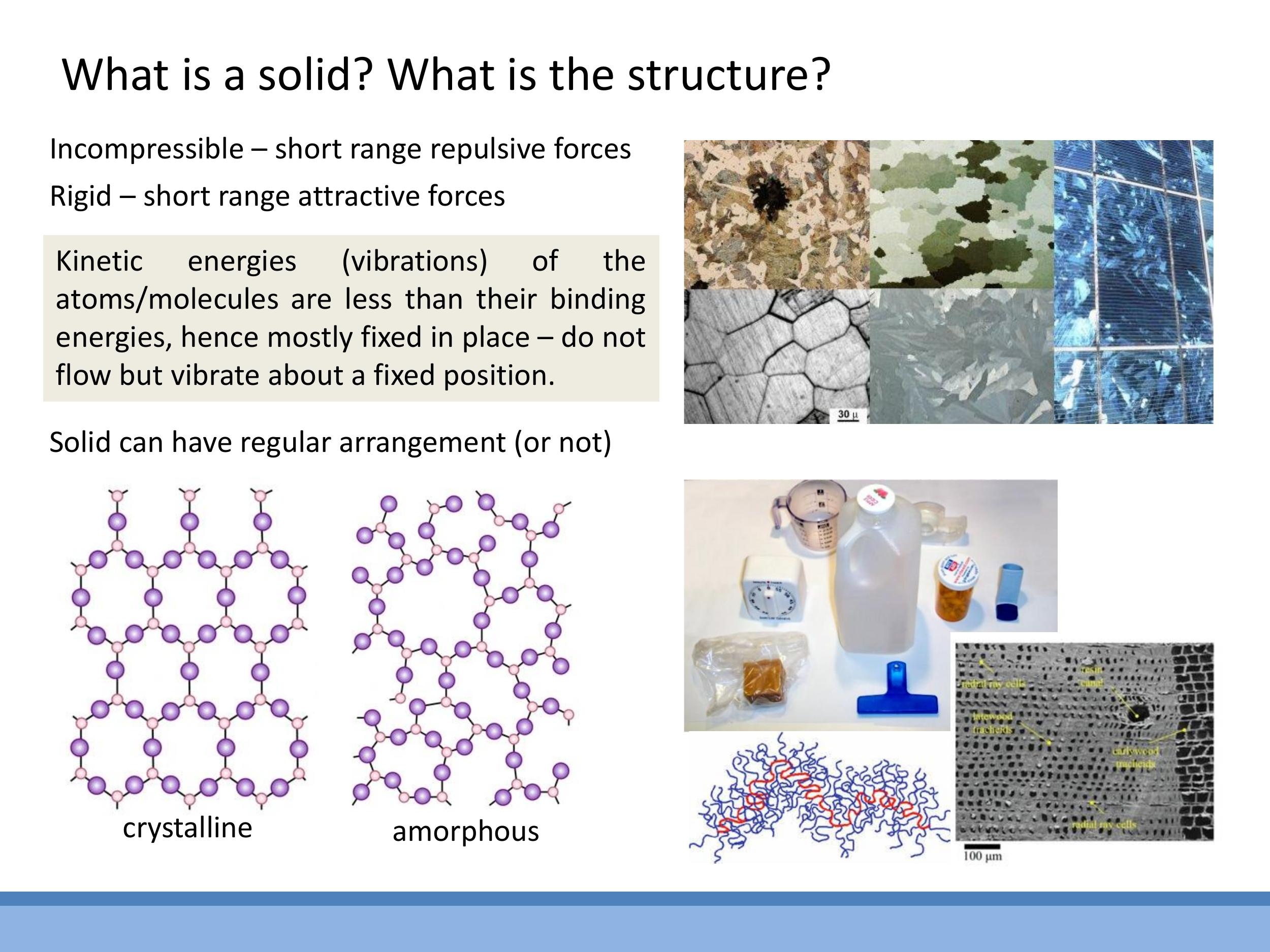
Macroscopically, a solid is defined by two key properties: it is incompressible and rigid
From a microscopic perspective, the distinguishing feature of a solid is that the kinetic energies of its constituent atoms are less than their binding energies. This means atoms in a solid do not exhibit translational motion, so there is no flow. Instead, their kinetic energy is solely in the form of vibrations around fixed equilibrium positions. This contrasts with liquids, where atomic kinetic energies are comparable to bonding energies, allowing molecules to move past their neighbours and rearrange.
2) Crystalline vs amorphous; grains and real materials
Solids can be broadly categorised into two structural classes: crystalline and amorphous. Crystalline solids possess a periodic, repeating arrangement of atoms, where each atom experiences the same local environment. In contrast, amorphous solids have atoms that are fixed in place but lack long-range periodicity, appearing more randomly arranged. Common examples of amorphous solids include polymers like plastics, wood, and glass.
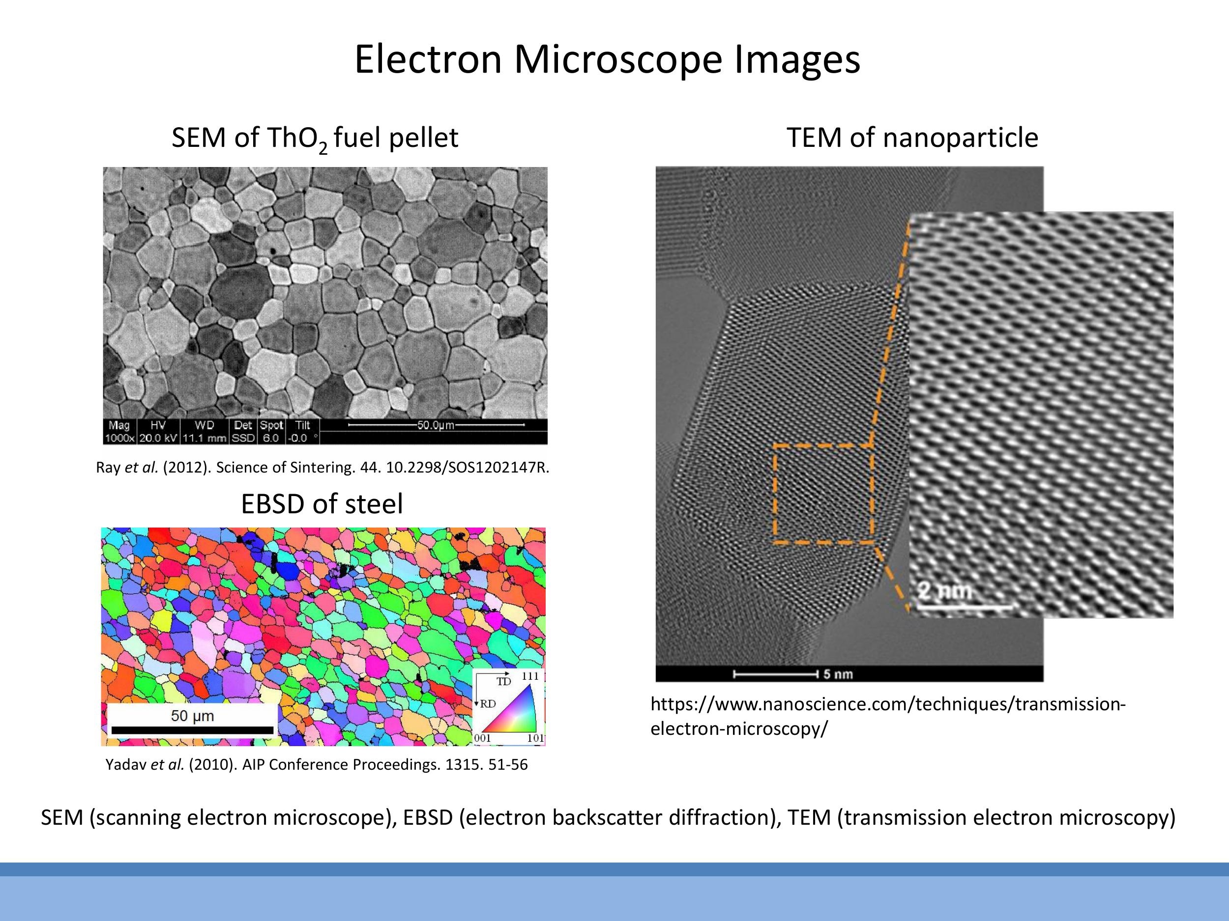
Most everyday crystalline materials are not perfect single crystals but are polycrystalline
The internal structure of materials can be visualised experimentally using electron microscopy. Techniques like Scanning Electron Microscopy (SEM) and Electron Backscatter Diffraction (EBSD) can reveal the size and orientation of grains at the micron scale. Transmission Electron Microscopy (TEM) offers even higher resolution, capable of showing atomic rows within a single grain, providing direct evidence of the perfect periodicity of atomic arrangements.
3) Packing atoms as spheres in 2D: from square to hexagonal
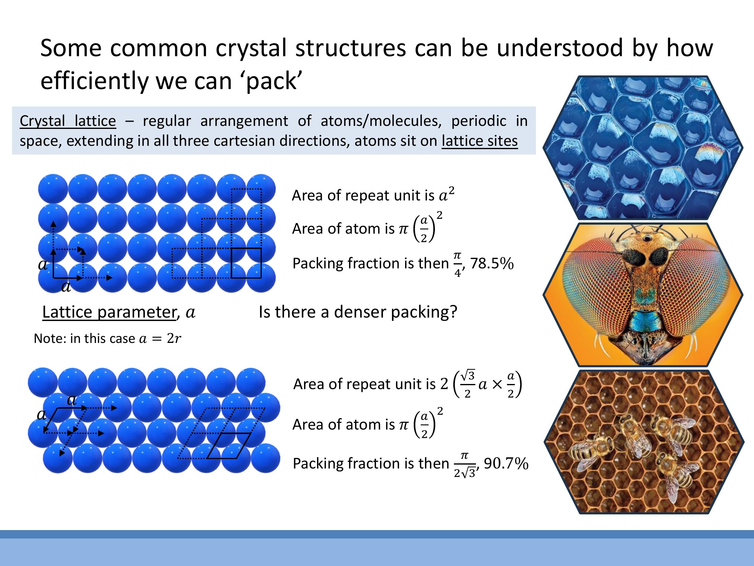
To understand crystal structures, we can model atoms as identical hard spheres and investigate how densely they can pack together. A key parameter in this analysis is the lattice parameter $a$, which defines the repeat distance between equivalent sites in the crystal.
Consider a square (simple) 2D lattice
$$
\text{Packing fraction} = \frac{\pi r^2}{a^2} = \frac{\pi r^2}{(2r)^2} = \frac{\pi r^2}{4r^2} = \frac{\pi}{4} \approx 78.5\%
$$
A denser arrangement is the hexagonal 2D lattice
$$
\text{Packing fraction} = \frac{\pi r^2}{\left(2 \times \frac{\sqrt{3}}{2} a \times r\right)} = \frac{\pi r^2}{(\sqrt{3} (2r) r)} = \frac{\pi r^2}{2\sqrt{3}r^2} = \frac{\pi}{2\sqrt{3}} \approx 90.7\%
$$
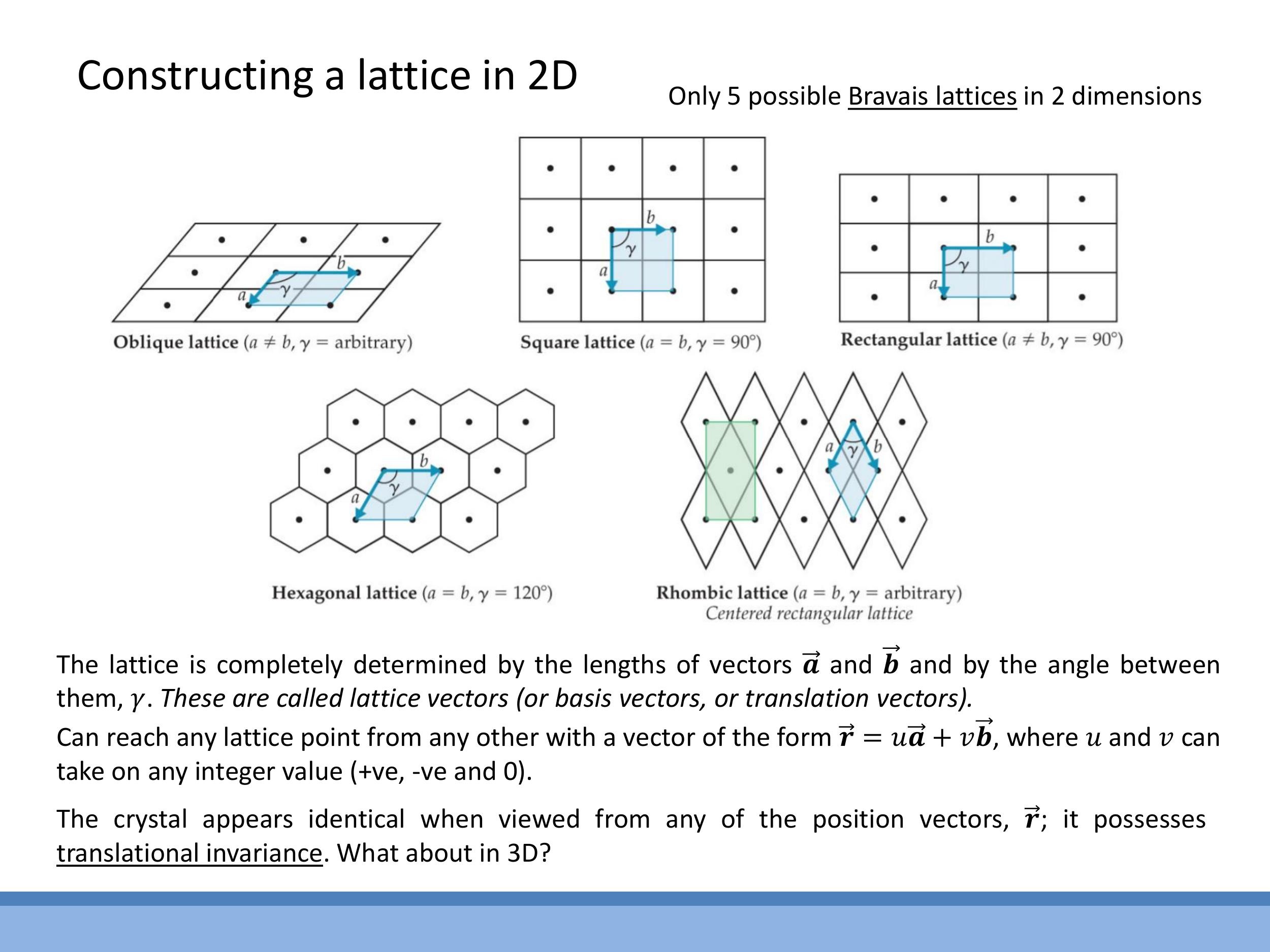
Crystal lattices exhibit translational invariance, meaning that any lattice point can be reached by taking integer steps along a set of basis vectors, and the structure appears identical from any of these points. In two dimensions, there are only five possible 2D Bravais lattices that satisfy this condition: oblique, square, rectangular, hexagonal, and rhombic (also known as centred rectangular).
4) From 2D layers to 3D close packing: hcp and fcc
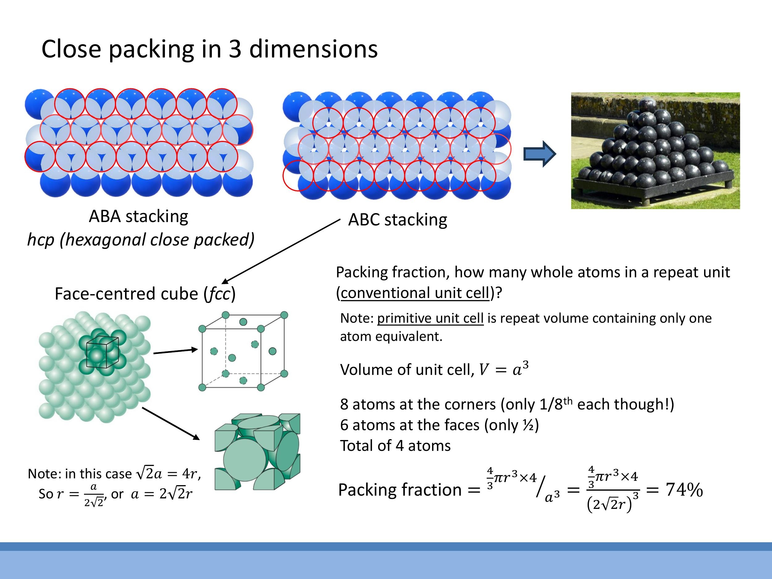
Extending the packing concept to three dimensions begins with a hexagonally packed layer of atoms. The spheres in the next layer sit in the gaps of the layer below, creating a denser arrangement. This "layer logic" leads to two common close-packed structures depending on the stacking sequence.
The first sequence is ABAB... stacking, where the third layer is positioned directly above the first. This arrangement results in a hexagonal close-packed (hcp) structure. The second sequence is ABCABC... stacking, where the third layer occupies a new set of gaps, different from both the first and second layers. This leads to a face-centred cubic (fcc) structure.
Both hcp and fcc structures achieve the densest possible sphere packing in three dimensions, sharing the same maximum packing fraction. For the purposes of calculations in this course, we will primarily focus on cubic structures.
5) The three cubic Bravais lattices; coordination and unit cells
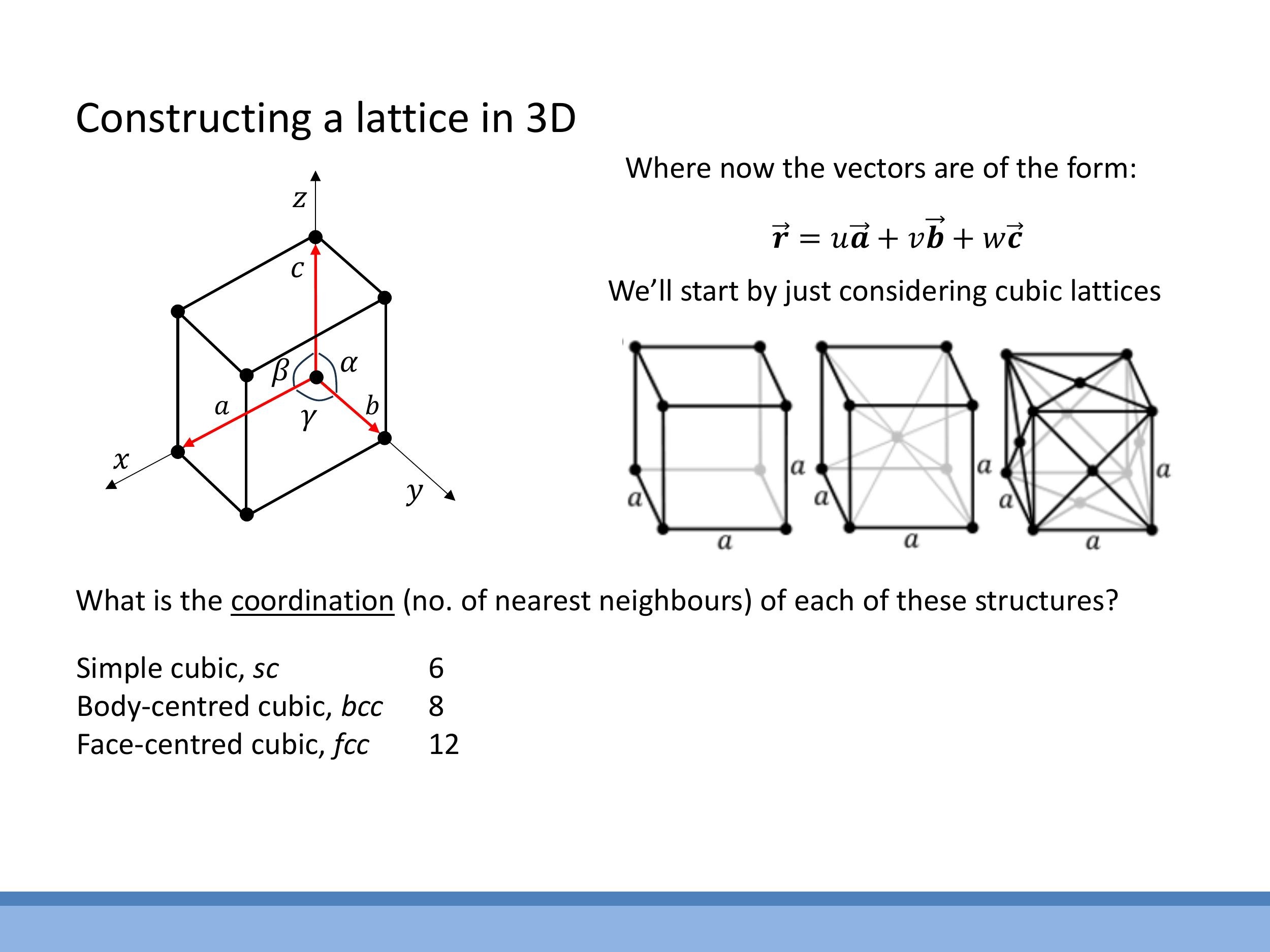
In three dimensions, the cubic system includes three primary Bravais lattices, each defined by an edge length $a$:
- Simple cubic (sc): Atoms are located only at the corners of the cube. This arrangement is rare in nature and is highly inefficient in terms of packing.
- Body-centred cubic (bcc): In addition to atoms at the corners, there is one atom located at the very centre of the cube. Iron (Fe) at certain temperatures exhibits this structure.
- Face-centred cubic (fcc): This structure features atoms at each corner of the cube and one atom at the centre of each of the six faces. Copper (Cu) is a classic example of an fcc metal.
The coordination number refers to the number of nearest neighbours to any given atom within the lattice. For these cubic structures, the coordination numbers are:
- Simple cubic (sc): $6$
- Body-centred cubic (bcc): $8$
- Face-centred cubic (fcc): $12$
It's important to distinguish between conventional unit cells and primitive unit cells
6) Worked density result: fcc packing fraction ≈ 74%
Let's calculate the packing fraction for the face-centred cubic (fcc) structure. First, we need to relate the lattice parameter $a$ to the atomic radius $r$. In an fcc lattice, the spheres touch along the face diagonal. The length of a face diagonal is $\sqrt{2} a$. This diagonal spans four atomic radii ($r + 2r + r$). Therefore, we have the relationship:
$$
\sqrt{2} a = 4r \implies a = 2\sqrt{2} r
$$
Next, we determine the number of atoms per conventional fcc unit cell. Each of the $8$ corner atoms contributes $\frac{1}{8}$ of an atom to the cell, and each of the $6$ face-centred atoms contributes $\frac{1}{2}$ of an atom. So, the total number of atoms per cell is:
$$
\left(8 \times \frac{1}{8}\right) + \left(6 \times \frac{1}{2}\right) = 1 + 3 = 4 \text{ atoms}
$$
Now we can calculate the packing fraction. This is the ratio of the total volume occupied by atoms within the cell to the total volume of the cell.
$$
\text{Packing fraction} = \frac{\text{Total atomic volume in cell}}{\text{Cell volume}} = \frac{4 \times \left(\frac{4}{3}\pi r^3\right)}{a^3}
$$
Substituting the expression for $a$ in terms of $r$:
$$
\text{Packing fraction} = \frac{\frac{16}{3}\pi r^3}{(2\sqrt{2} r)^3} = \frac{\frac{16}{3}\pi r^3}{16\sqrt{2} r^3} = \frac{\pi}{3\sqrt{2}} \approx 0.74
$$
This means the fcc packing fraction is approximately $74 \% $. It's important to note that the hexagonal close-packed (hcp) structure has the same packing fraction, as both are considered close-packed arrangements.
7) The classification landscape: 7 crystal systems and 14 Bravais lattices
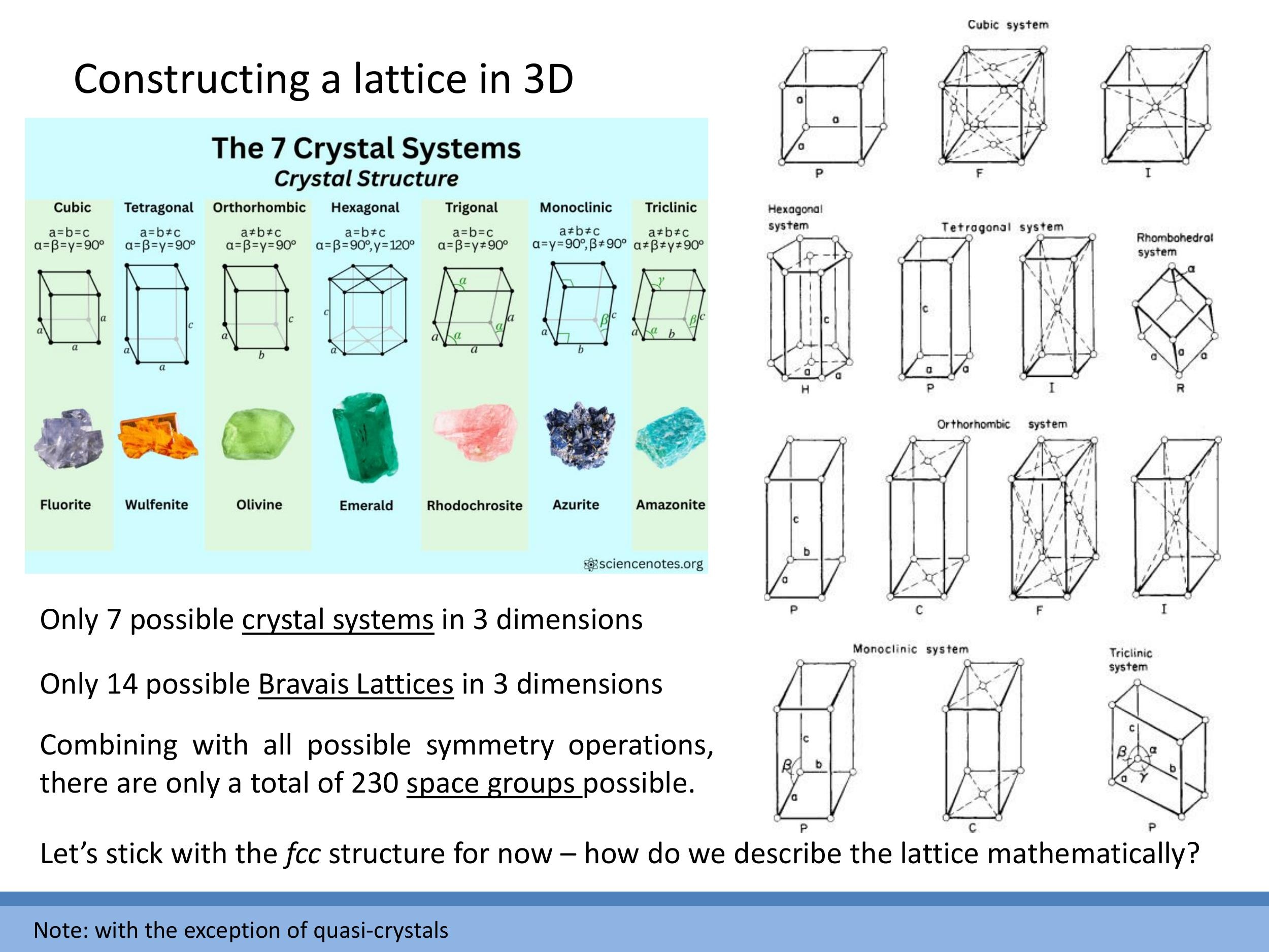
Beyond the specific cubic examples, there is a comprehensive classification system for all three-dimensional crystal structures. All crystals can be categorised into one of 7 crystal systems, which are defined by the relationships between their lattice parameters (edge lengths $a$, $b$, $c$) and interaxial angles ($\alpha$, $\beta$, $\gamma$). These systems include cubic, tetragonal, orthorhombic, hexagonal, trigonal, monoclinic, and triclinic.
Within these 7 crystal systems, there are a total of 14 Bravais lattices
When these 14 Bravais lattices are further combined with all possible symmetry operations (such as mirror planes and glide planes), they yield a total of 230 space groups
8) Hands-on observation: macroscopic crystal shapes reflect symmetry
During the lecture, several physical crystals were passed around, including iron pyrite (often called "fool's gold," which exhibits a cubic crystal system), quartz, and selenite. Additionally, models of face-centred cubic (fcc) and body-centred cubic (bcc) structures were shown. This demonstration illustrated that slowly grown crystals often display external faces that are consistent with their internal atomic symmetry. For example, cubic crystals like iron pyrite tend to form visible cube-shaped external faces.
Slides present but not covered this lecture (for clarity)
The concepts of directions and planes using Miller indices were introduced in the slides but explicitly deferred by the lecturer. This material, including slides PoM_lecture_14_page_10.jpg, PoM_lecture_14_page_11.jpg, PoM_lecture_14_page_12.jpg, and PoM_lecture_14_page_13.jpg, will be covered in a subsequent lecture and has not been included in the prose for this lecture.
Appendix: Bragg’s law and measuring lattice spacings (supplementary)
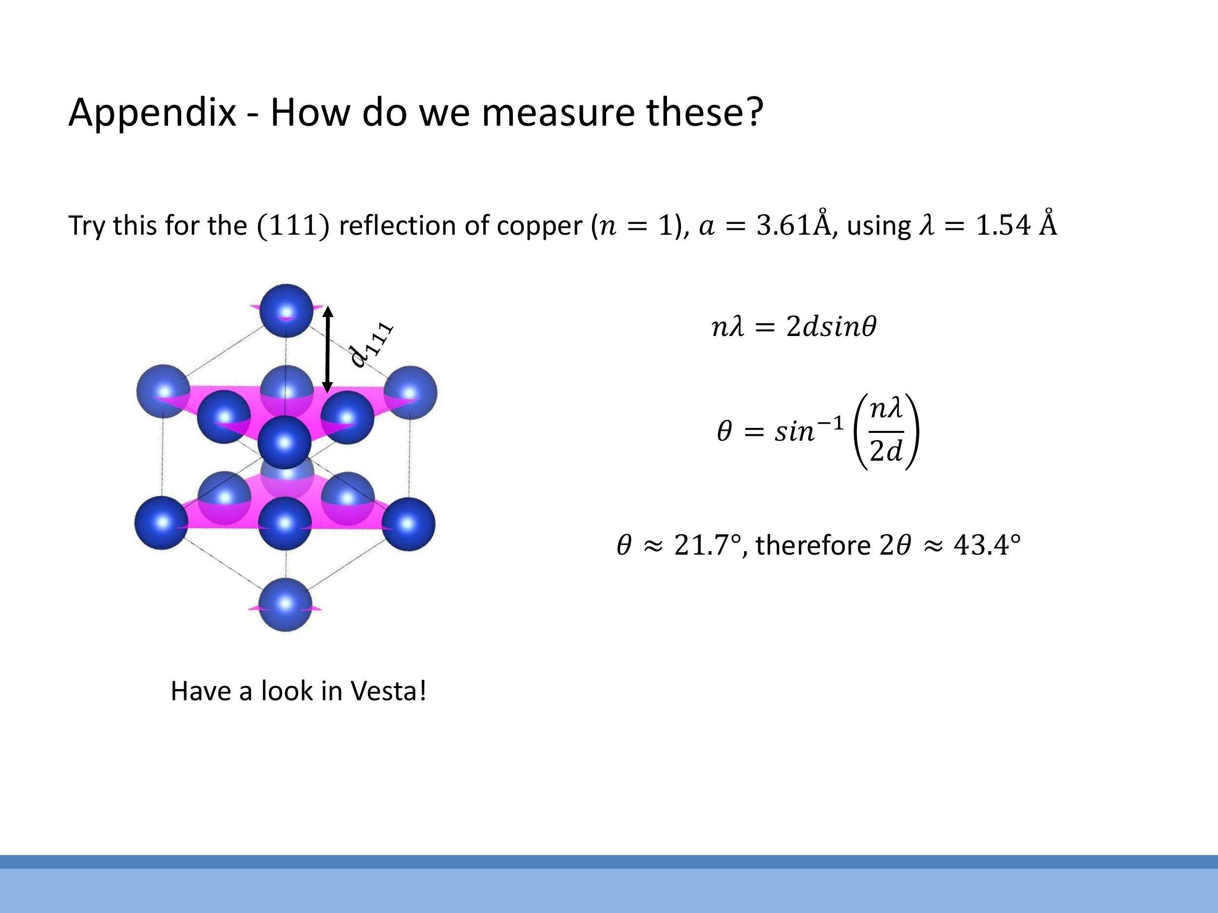
Side Note: This material is supplementary and won't be examined, but provides useful context.
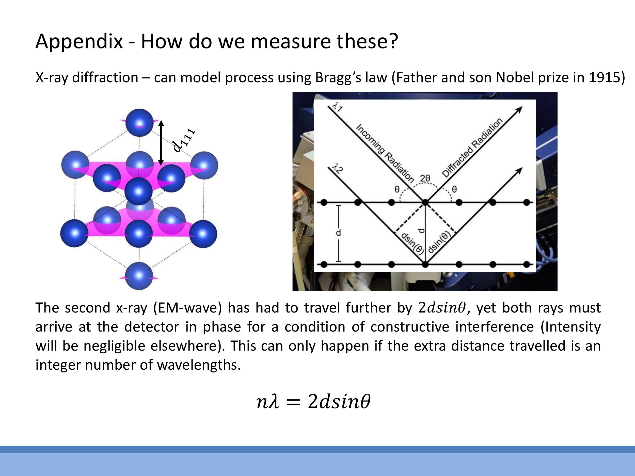
X-ray diffraction is a powerful experimental technique that allows us to determine the interplanar spacings $d$ within a crystal lattice, using Bragg’s law: $n\lambda = 2d \sin\theta$. This equation relates the wavelength $\lambda$ of the X-rays, the diffraction angle $\theta$, and an integer $n$ representing the order of diffraction. In practice, X-ray diffraction is typically used to identify which crystallographic planes (indexed as $(hkl)$) diffract at specific angles $\theta$ for a given X-ray wavelength $\lambda$. From these measurements, the interplanar spacing $d$ can be inferred, which in turn helps to determine the lattice parameters of the crystal. For example, observing the $(111)$ reflection of copper with a known wavelength of approximately $1.54 \, \text{Å}$ allows us to determine its face-centred cubic (fcc) spacing relationships.
Key takeaways
Solids are incompressible and rigid because steep short-range repulsive forces prevent compression, while attractive forces hold atoms in fixed positions. At a microscopic level, atoms in a solid vibrate about these fixed positions, lacking the translational motion found in liquids.
Crystalline solids are characterised by a long-range periodic order in their atomic arrangement, whereas amorphous solids lack this extended periodicity. Most real-world crystalline materials are polycrystalline, meaning they are composed of many small, oriented crystalline grains.
Modelling atoms as spheres helps to build intuition about packing efficiency. In two dimensions, square packing achieves approximately $78.5 \% $ efficiency, while hexagonal packing is denser at roughly $ 90.7 \% $. In three dimensions, close packing formed by stacking hexagonal layers leads to either hexagonal close-packed (hcp) or face-centred cubic (fcc) structures, both achieving a maximum packing efficiency of approximately $ 74 \% $.
The three cubic Bravais lattices are simple cubic (sc), body-centred cubic (bcc), and face-centred cubic (fcc), with coordination numbers (number of nearest neighbours) of $6$, $8$, and $12$ respectively. For the fcc structure, the lattice parameter $a$ is related to the atomic radius $r$ by $\sqrt{2} a = 4r$, and its packing fraction is approximately $74 \% $.
Beyond the cubic system, there are $7$ distinct crystal systems and $14$ Bravais lattices that describe all possible three-dimensional periodic arrangements of atoms. When combined with various symmetry operations, these lattices give rise to $230$ unique space groups.
The content on Miller indices was deferred to the next lecture, and Bragg's law, presented in the appendix, is for general interest only and will not be examinable this year.
## Lecture 14: Solids and Crystals
### 0) Orientation, admin, and learning outcomes
There are a few administrative updates for the course. The problems class scheduled for Friday has been cancelled. Instead, a two-hour revision session will take place next week, covering both Mechanics and Properties of Matter. This session will be recorded. During the revision, the lecturer will highlight specific slides and topics that are typically relevant to exam-style questions, particularly for the December test, which consists of ten multiple-choice questions.
This lecture marks a shift in our focus, moving back from thermodynamics to the phases of matter, specifically concentrating on solids.
By the end of this lecture, you should be able to define and characterise a solid, define a crystal, recall that there are $7$ crystal systems and $14$ Bravais lattices (without needing to memorise all of them at this stage), draw and describe the three cubic Bravais lattices (simple cubic, body-centred cubic, and face-centred cubic), and calculate packing fractions for these structures.
### 1) What is a solid? Macroscopic properties and microscopic picture

Macroscopically, a solid is defined by two key properties: it is **incompressible** and **rigid**. Its incompressibility arises from steep short-range repulsive forces between atoms, which make it very difficult to squeeze them closer together. Its rigidity is due to net attractive forces that hold the atoms in fixed positions, resisting any shear or flow.
From a microscopic perspective, the distinguishing feature of a solid is that the kinetic energies of its constituent atoms are less than their binding energies. This means atoms in a solid do not exhibit translational motion, so there is no flow. Instead, their kinetic energy is solely in the form of vibrations around fixed equilibrium positions. This contrasts with liquids, where atomic kinetic energies are comparable to bonding energies, allowing molecules to move past their neighbours and rearrange.
### 2) Crystalline vs amorphous; grains and real materials


Solids can be broadly categorised into two structural classes: crystalline and amorphous. **Crystalline solids** possess a periodic, repeating arrangement of atoms, where each atom experiences the same local environment. In contrast, **amorphous solids** have atoms that are fixed in place but lack long-range periodicity, appearing more randomly arranged. Common examples of amorphous solids include polymers like plastics, wood, and glass.
Most everyday crystalline materials are not perfect single crystals but are **polycrystalline**. This means they are composed of many small single-crystal regions, or "grains," each with a different crystallographic orientation, mosaicked together. For instance, the glinting effect seen on steel railings in the sun is caused by light reflecting off these differently oriented crystallographic grains within the steel.
The internal structure of materials can be visualised experimentally using electron microscopy. Techniques like Scanning Electron Microscopy (SEM) and Electron Backscatter Diffraction (EBSD) can reveal the size and orientation of grains at the micron scale. Transmission Electron Microscopy (TEM) offers even higher resolution, capable of showing atomic rows within a single grain, providing direct evidence of the perfect periodicity of atomic arrangements.
### 3) Packing atoms as spheres in 2D: from square to hexagonal

To understand crystal structures, we can model atoms as identical hard spheres and investigate how densely they can pack together. A key parameter in this analysis is the **lattice parameter** $a$, which defines the repeat distance between equivalent sites in the crystal.
Consider a **square (simple) 2D lattice**. In this arrangement, the atoms form a simple square grid where the lattice parameter $a = 2r$, with $r$ being the atomic radius. A conventional unit cell for this lattice is a square containing one atom (from $4$ corners $\times$ $\frac{1}{4}$ atom per corner). The packing fraction, representing the ratio of the area occupied by atoms to the total area of the cell, is calculated as:
$$ \text{Packing fraction} = \frac{\pi r^2}{a^2} = \frac{\pi r^2}{(2r)^2} = \frac{\pi r^2}{4r^2} = \frac{\pi}{4} \approx 78.5\% $$
A denser arrangement is the **hexagonal 2D lattice**. Here, atoms are packed more closely, with rows shifted to fill the gaps. The repeat unit is a parallelogram composed of two equilateral triangles, which still contains one atom equivalent. The packing fraction for this arrangement is significantly higher:
$$ \text{Packing fraction} = \frac{\pi r^2}{\left(2 \times \frac{\sqrt{3}}{2} a \times r\right)} = \frac{\pi r^2}{(\sqrt{3} (2r) r)} = \frac{\pi r^2}{2\sqrt{3}r^2} = \frac{\pi}{2\sqrt{3}} \approx 90.7\% $$
Crystal lattices exhibit **translational invariance**, meaning that any lattice point can be reached by taking integer steps along a set of basis vectors, and the structure appears identical from any of these points. In two dimensions, there are only five possible **2D Bravais lattices** that satisfy this condition: oblique, square, rectangular, hexagonal, and rhombic (also known as centred rectangular).

### 4) From 2D layers to 3D close packing: hcp and fcc

Extending the packing concept to three dimensions begins with a hexagonally packed layer of atoms. The spheres in the next layer sit in the gaps of the layer below, creating a denser arrangement. This "layer logic" leads to two common close-packed structures depending on the stacking sequence.
The first sequence is **ABAB... stacking**, where the third layer is positioned directly above the first. This arrangement results in a **hexagonal close-packed (hcp)** structure. The second sequence is **ABCABC... stacking**, where the third layer occupies a new set of gaps, different from both the first and second layers. This leads to a **face-centred cubic (fcc)** structure.
Both hcp and fcc structures achieve the densest possible sphere packing in three dimensions, sharing the same maximum packing fraction. For the purposes of calculations in this course, we will primarily focus on cubic structures.
### 5) The three cubic Bravais lattices; coordination and unit cells

In three dimensions, the cubic system includes three primary Bravais lattices, each defined by an edge length $a$:
* **Simple cubic (sc):** Atoms are located only at the corners of the cube. This arrangement is rare in nature and is highly inefficient in terms of packing.
* **Body-centred cubic (bcc):** In addition to atoms at the corners, there is one atom located at the very centre of the cube. Iron (Fe) at certain temperatures exhibits this structure.
* **Face-centred cubic (fcc):** This structure features atoms at each corner of the cube and one atom at the centre of each of the six faces. Copper (Cu) is a classic example of an fcc metal.
The **coordination number** refers to the number of nearest neighbours to any given atom within the lattice. For these cubic structures, the coordination numbers are:
* Simple cubic (sc): $6$
* Body-centred cubic (bcc): $8$
* Face-centred cubic (fcc): $12$
It's important to distinguish between **conventional unit cells** and **primitive unit cells**. The conventional cell is the obvious cube, including corner atoms and any face or body-centre atoms, and is typically used for cubic metals due to its intuitive nature. A primitive cell, however, is the smallest volume unit that contains the equivalent of only one atom, and it is usually less intuitive to visualise for cubic systems.
### 6) Worked density result: fcc packing fraction ≈ 74%

Let's calculate the packing fraction for the face-centred cubic (fcc) structure. First, we need to relate the lattice parameter $a$ to the atomic radius $r$. In an fcc lattice, the spheres touch along the face diagonal. The length of a face diagonal is $\sqrt{2} a$. This diagonal spans four atomic radii ($r + 2r + r$). Therefore, we have the relationship:
$$ \sqrt{2} a = 4r \implies a = 2\sqrt{2} r $$
Next, we determine the number of atoms per conventional fcc unit cell. Each of the $8$ corner atoms contributes $\frac{1}{8}$ of an atom to the cell, and each of the $6$ face-centred atoms contributes $\frac{1}{2}$ of an atom. So, the total number of atoms per cell is:
$$ \left(8 \times \frac{1}{8}\right) + \left(6 \times \frac{1}{2}\right) = 1 + 3 = 4 \text{ atoms} $$
Now we can calculate the packing fraction. This is the ratio of the total volume occupied by atoms within the cell to the total volume of the cell.
$$ \text{Packing fraction} = \frac{\text{Total atomic volume in cell}}{\text{Cell volume}} = \frac{4 \times \left(\frac{4}{3}\pi r^3\right)}{a^3} $$
Substituting the expression for $a$ in terms of $r$:
$$ \text{Packing fraction} = \frac{\frac{16}{3}\pi r^3}{(2\sqrt{2} r)^3} = \frac{\frac{16}{3}\pi r^3}{16\sqrt{2} r^3} = \frac{\pi}{3\sqrt{2}} \approx 0.74 $$
This means the fcc packing fraction is approximately $74\%$. It's important to note that the hexagonal close-packed (hcp) structure has the same packing fraction, as both are considered close-packed arrangements.
### 7) The classification landscape: 7 crystal systems and 14 Bravais lattices

Beyond the specific cubic examples, there is a comprehensive classification system for all three-dimensional crystal structures. All crystals can be categorised into one of **7 crystal systems**, which are defined by the relationships between their lattice parameters (edge lengths $a$, $b$, $c$) and interaxial angles ($\alpha$, $\beta$, $\gamma$). These systems include cubic, tetragonal, orthorhombic, hexagonal, trigonal, monoclinic, and triclinic.
Within these 7 crystal systems, there are a total of **14 Bravais lattices**. These represent the only ways to arrange points in three-dimensional space such that the arrangement is translationally equivalent from any point, maintaining the inherent symmetry of the lattice.
When these 14 Bravais lattices are further combined with all possible symmetry operations (such as mirror planes and glide planes), they yield a total of **230 space groups**. This advanced classification provides a complete description of all possible periodic crystal structures.
### 8) Hands-on observation: macroscopic crystal shapes reflect symmetry
During the lecture, several physical crystals were passed around, including iron pyrite (often called "fool's gold," which exhibits a cubic crystal system), quartz, and selenite. Additionally, models of face-centred cubic (fcc) and body-centred cubic (bcc) structures were shown. This demonstration illustrated that slowly grown crystals often display external faces that are consistent with their internal atomic symmetry. For example, cubic crystals like iron pyrite tend to form visible cube-shaped external faces.
### Slides present but not covered this lecture (for clarity)
The concepts of directions and planes using Miller indices were introduced in the slides but explicitly deferred by the lecturer. This material, including slides `PoM_lecture_14_page_10.jpg`, `PoM_lecture_14_page_11.jpg`, `PoM_lecture_14_page_12.jpg`, and `PoM_lecture_14_page_13.jpg`, will be covered in a subsequent lecture and has not been included in the prose for this lecture.
## Appendix: Bragg’s law and measuring lattice spacings (supplementary)


> *Side Note:* This material is supplementary and won't be examined, but provides useful context.
X-ray diffraction is a powerful experimental technique that allows us to determine the interplanar spacings $d$ within a crystal lattice, using **Bragg’s law**: $n\lambda = 2d \sin\theta$. This equation relates the wavelength $\lambda$ of the X-rays, the diffraction angle $\theta$, and an integer $n$ representing the order of diffraction. In practice, X-ray diffraction is typically used to identify which crystallographic planes (indexed as $(hkl)$) diffract at specific angles $\theta$ for a given X-ray wavelength $\lambda$. From these measurements, the interplanar spacing $d$ can be inferred, which in turn helps to determine the lattice parameters of the crystal. For example, observing the $(111)$ reflection of copper with a known wavelength of approximately $1.54\,\text{Å}$ allows us to determine its face-centred cubic (fcc) spacing relationships.
## Key takeaways
Solids are incompressible and rigid because steep short-range repulsive forces prevent compression, while attractive forces hold atoms in fixed positions. At a microscopic level, atoms in a solid vibrate about these fixed positions, lacking the translational motion found in liquids.
Crystalline solids are characterised by a long-range periodic order in their atomic arrangement, whereas amorphous solids lack this extended periodicity. Most real-world crystalline materials are polycrystalline, meaning they are composed of many small, oriented crystalline grains.
Modelling atoms as spheres helps to build intuition about packing efficiency. In two dimensions, square packing achieves approximately $78.5\%$ efficiency, while hexagonal packing is denser at roughly $90.7\%$. In three dimensions, close packing formed by stacking hexagonal layers leads to either hexagonal close-packed (hcp) or face-centred cubic (fcc) structures, both achieving a maximum packing efficiency of approximately $74\%$.
The three cubic Bravais lattices are simple cubic (sc), body-centred cubic (bcc), and face-centred cubic (fcc), with coordination numbers (number of nearest neighbours) of $6$, $8$, and $12$ respectively. For the fcc structure, the lattice parameter $a$ is related to the atomic radius $r$ by $\sqrt{2} a = 4r$, and its packing fraction is approximately $74\%$.
Beyond the cubic system, there are $7$ distinct crystal systems and $14$ Bravais lattices that describe all possible three-dimensional periodic arrangements of atoms. When combined with various symmetry operations, these lattices give rise to $230$ unique space groups.
The content on Miller indices was deferred to the next lecture, and Bragg's law, presented in the appendix, is for general interest only and will not be examinable this year.